what is the meaning of overfitting

Overfitting is strongly related to variable selection. It is a common problem and a tough one, best explained by way of example.

Assume the real unknown model is

$y_t = x_{1t}+x_{2t} + \varepsilon_t,$

we do not know that it is only those two variables that matter, and in fact we have 10 potential variables:

$\{x_{it}\}^{10}_{i = 1}.$

So we fit. I first generate/simulate the two important variables, generate random noise, add 8 unimportant variables and estimate the regression:


TT=500
x1 = rnorm(TT)
x2 = rnorm(TT)
eps <- rnorm(TT)
y = x1+x2+eps # The real unknown model
summary(lm(y~x1+x2))
P = 10
rest <- matrix(nrow = TT, ncol = P)
for (i in 3:10){ # Simulate 8 more variables which are NOT relevant 
  rest[,i] <- rnorm(TT)
}
X <- cbind(x1,x2,rest[,3:10])
colnames(X) <- 1:10

lm0 <- (lm(y~X)) 
library(stargazer) # for the next function
htmlreg(lm0, single.row = T,caption = "Coefficient's Value",stars = 0.05, 
html.tag=T,bold = 0.05 , caption.above = T, center = T, inline.css = T)

TT=500

x1 = rnorm(TT)

x2 = rnorm(TT)

eps <- rnorm(TT)

y = x1+x2+eps # The real unknown model

summary(lm(y~x1+x2))

P = 10

rest <- matrix(nrow = TT, ncol = P)

for (i in 3:10){ # Simulate 8 more variables which are NOT relevant

rest[,i] <- rnorm(TT)

}

X <- cbind(x1,x2,rest[,3:10])

colnames(X) <- 1:10

lm0 <- (lm(y~X))

library(stargazer) # for the next function

htmlreg(lm0, single.row = T,caption = "Coefficient's Value",stars = 0.05,

html.tag=T,bold = 0.05 , caption.above = T, center = T, inline.css = T)

You can see that also variables number 3 and 10 seem to be important (even though we know they are not). Such a simple setting.. with 500 observations.. and this unwelcome result. What happened??

Coefficient’s Value
	Bold means significant
(Intercept)	-0.07 (0.05)
X1	1.01 (0.05)^*
X2	0.98 (0.05)^*
X3	-0.09 (0.05)^*
X4	0.02 (0.05)
X5	0.05 (0.05)
X6	-0.02 (0.05)
X7	0.04 (0.05)
X8	-0.07 (0.05)
X9	0.01 (0.05)
X10	0.10 (0.05)^*
R²	0.65
Adj. R²	0.65
Num. obs.	500
^*p < 0.05

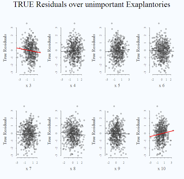
Once the simple model easily discovered that variables 1 and 2 are important, we were unlucky. In this toy example we know what are the true residuals. It appears that these residuals, the true residuals, can be made smaller, just by chance using variables 3 and 10. That is, the computer discovered that if it adds those unimportant variables it can substantially decrease the residuals further. We know that the residuals should ‘stay put’, but the incidental correlation is too strong to be ignored.

I regress the real (known to us) residuals on each of the unimportant (known to us) variables. Since we repeat this check 8 times, there is a very high chance to end up with at least one more ‘important’ unimportant:


for (i in 3:P){
  plot(eps~X[,i], xlab = paste("x",i), ylab = "True Residuals",cex.lab = 1.7)
# The next line asks to color the fit if it is significant:
  col1 <- lwd1 <- ifelse(summary(lm(y~X))$coef[i+1,4]<.05,2,1)
  abline(lm(eps~X[,i]),col=col1,lwd=lwd1)
}
title(main = "TRUE Residuals over unimportant Exaplantories",
outer = T,  cex.main = 3)

for (i in 3:P){

plot(eps~X[,i], xlab = paste("x",i), ylab = "True Residuals",cex.lab = 1.7)

# The next line asks to color the fit if it is significant:

col1 <- lwd1 <- ifelse(summary(lm(y~X))$coef[i+1,4]<.05,2,1)

abline(lm(eps~X[,i]),col=col1,lwd=lwd1)

}

title(main = "TRUE Residuals over unimportant Exaplantories",

outer = T, cex.main = 3)

The plot shows the fit from the 8 individual regressions:

This is what we mean when we sometimes say “fitting the noise in the data”. It has consequences both in inference, when you report nonsense to your boss (or to the world), and in prediction. These two ‘false’ variables will worsen out-of-sample performance if used for prediction.

As a next level bullet-point, I stress the importance of an underlying model; include interest rate as explanatory for the level of investment (even if insignificant) and fear not to exclude significant variables that make little sense to you (even if they are significant).

Coefficient’s Value
	Model 1
(Intercept)	-0.04 (0.05)
X1	1.05 (0.05)^*
X2	0.98 (0.05)^*
X3	0.09 (0.05)
X4	0.03 (0.05)
X5	-0.06 (0.05)
X6	-0.06 (0.05)
X7	-0.11 (0.05)^*
X8	0.02 (0.05)
X9	0.02 (0.05)
X10	0.03 (0.05)
R²	0.67
Adj. R²	0.66
Num. obs.	500
^*p < 0.05

You might also like:

What is overfitting?

You might also like:

One comment on “What is overfitting?”

Leave a Reply