Piecewise Regression

A beta of a stock generally means its relation with the market, how many percent move we should expect from the stock when the market moves one percent.

Market, being a somewhat vague notion is approximated here, as usual, using the S&P 500. This aforementioned relation (henceforth, beta) is detrimental to many aspects of trading and risk management. It is already well established that volatility has different dynamics for rising markets and for declining market. Recently, I read few papers that suggest the same holds true for beta, specifically that the beta is not the same for rising markets and for declining markets. We anyway use regression for estimation of beta, so piecewise linear regression can fit right in for an investor/speculator who wishes to accommodate himself with this asymmetry.

The idea is very simple, we divide the dataset into two (or more) parts and estimate each part separately, piece by piece, or piecewise. This simple idea can be made with complex notation and code, which is necessary when you move up in complexity level, the interested reader can google regression splines or check the references below.

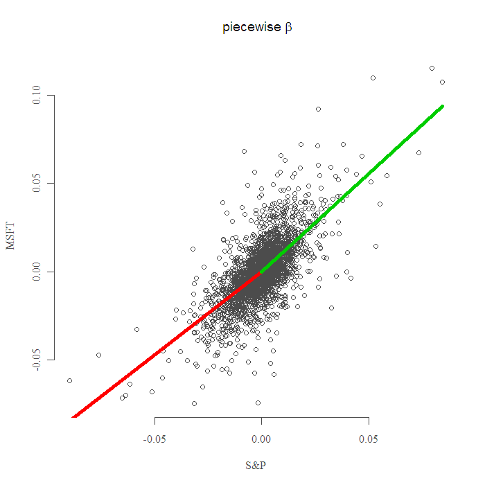
For illustration, I use Microsoft returns (MSFT). I estimate different beta‘s for green days and for red days, positive days are above zero and negative days are below zero, so zero is our breaking point. (The breaking point is called “knot” in academic jargon, why “knot”? maybe because it ties the two parts together, but probably so people on the outside will not be able to get it.) The following plot shows the result:

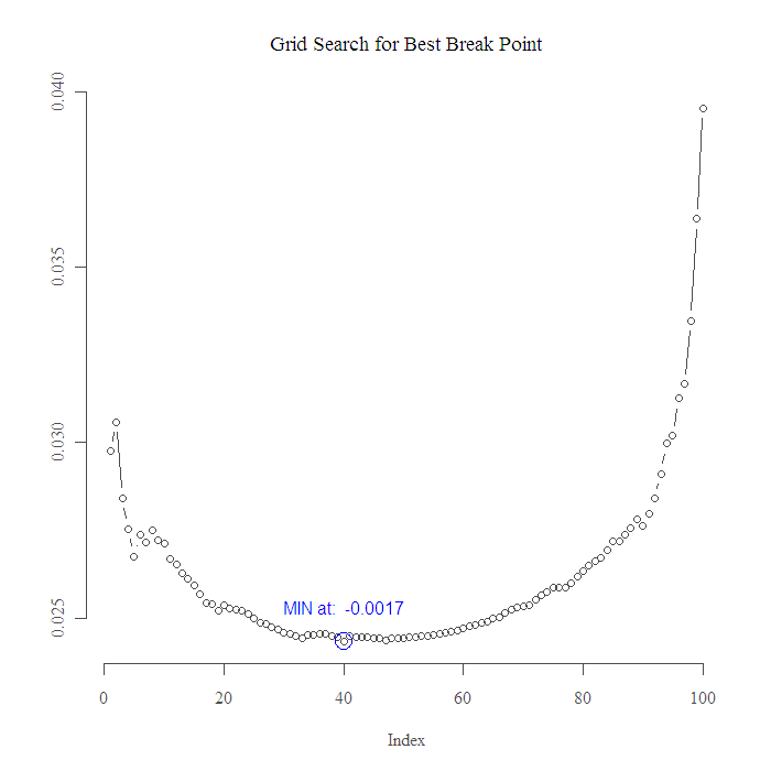
You know what? maybe it is not zero we should take as a break point, maybe the beta is the same all the way till the extreme negative, and only say when the market is moving sharply down, only then the relation changes. Let us ask the data. This falls under the category of structural change. I consider a grid of points along the axis, and build a model with a break at each point, one slope before the break another slope after the break. I look for the minimum of the Sum of Squared Errors over the whole sample, so I sum up the squared errors from the two models. The following figure shows the result:

Well, data says the breaking point is not zero, but it is almost zero, tough luck, all this work and for what I ask you? OK then, in order to use the correct beta all you have to do now is to decide, is it a bear market or a bull market.. should be a breeze. Thanks for reading, as always code is given below.

References:                                                                                                                      

Code:
Note that you can also use package “segmented” and package “strucchange”, both are extensive and suitable, but maybe it is better to code it yourself.