Forecasting the Misery Index, follow-up

Five months ago I generated forecasts for the Eurozone Misery index. I used the built-in “FitAR” package in R. Using different models differing in their memory length (how many lags were considered for each model) 24 months ahead forecasts were generated. Might be interesting to see how accurate are the forecasts. The previous post is updated and few bugs corrected in the code. The updated data is public and can be found here. It is the sum of inflation rate and unemployment rate in the Euro-zone area.

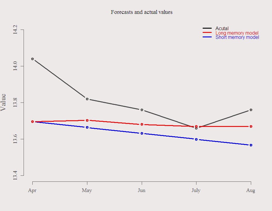
To preview the results, last post showed that the short memory models predict the index to decline while the long memory models predict it to stay at current relatively high levels. Five months later..

Well, (1) both models were surprised by the April jump in the index. (2) longer memory performed uniformly better. The July forecast could not be more accurate and it seems that indeed the econometric model captures Euro-zone issues quite well. The model does not let the index revert to its historical mean yet, which is consistent with the issues at hand (Greek debt etc.) as well as with Okun’s law, which is that output and employment commonly move together.

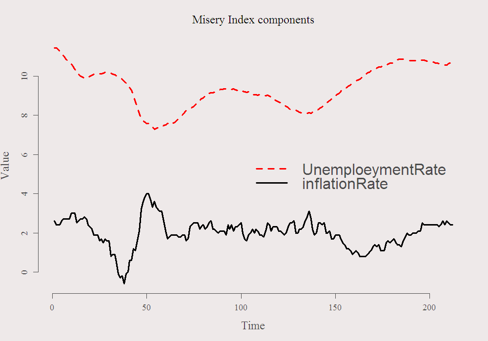
Empirically, unemployment tends to fall by 1 percentage point for every 3-percentage point rise in output. In the Euro-zone, output growth is weak these days. In accordance with the Keynesian multiplier, it draws us down, and will keep on doing so in the near future. Implicitly, the claim here is that the index is struggling due to unemployment rate, and not because price level (inflation) is rising. See that it is the case:

We are looking at the very end of these curves. You can see the black line (inflation) declines slightly while the red (unemployment) rise. From September 2011, the inflation rate declined from 3% to 2.5% while unemployment rate rose from 10.34 to 11.44. Sticky unemployment indeed. As always, code is given below, for the data scroll up to the link made public. Thanks for reading.