This post is about the concept of entropy in the context of information-theory. Where does the term entropy comes from? What does it actually mean? And how does it clash with the notion of robustness?
Where does the term entropy (supposedly) come from?
The term entropy was imported to information theory by Claude Shannon. Pasted from “Entropy, von Neumann and the von Neumann entropy”, Shannon reportedly wrote in his 1971 paper Energy and information:
“My greatest concern was what to call it. I thought of calling it ‘information’, but the word was overly used, so I decided to call it ‘uncertainty’. When I discussed it with John von Neumann, he had a better idea. Von Neumann told me, ‘You should call it entropy, for two reasons. In the first place your uncertainty function has been used in statistical mechanics under that name, so it already has a name. In the second place, and more important, nobody knows what entropy really is, so in a debate you will always have the advantage.'”
Entropy as a measure of expected surprise – part 1
If a random variable x has what they call a degenerate distribution, that is, it takes the one value with probability 1, then there is no surprise. Think 1-sided dice, or a two-headed coin (both sides are ‘head’). Every draw results in the same value; so your guess is always going to be correct, zero surprise. In that case the entropy of that random variable is zero, which also tells you it’s not actually random.
If it is a regular coin toss, then both values (heads, tails) are equally likely. So from that point on it’s not possible to increase the amount of surprise. Your guess is of no help, with no way to make us useful. If it is a biased coin, say a larger chance to land on heads, then you can “help” your guess by declaring heads. Meaning that particular random variable (the coin toss) is less random, so less surprise is expected.
Formally we quantify entropy using Shannon’s entropy (but there are few more ways):
![\[S=-\sum _{i}P_{i}\log {P_{i}}\]](https://eranraviv.com/wp-content/ql-cache/quicklatex.com-0841b97d5e88ea0c5441b562c186e768_l3.svg "Rendered by QuickLaTeX.com")
Let’s zoom in.  is the probability of event
  . If we would lose the minus sign and instead of
  use would simply use the value of the event , say
  we would end up with the formula for the expectation of the random variable. So perhaps that is why we refer to it as “expected” surprise. Note also that we couldn’t care less about the value of , only about the probability, or frequency. The distinction between probability and frequency is important here. In reality we usually don’t know the probability, we estimate it from the frequency we observe. Here is some code to complement the above explanation:
> # Degenerated distribution
> x <- rep("head", 2)
> p <- table(x)/length(x)
> -sum( p * log2(p) )
[1] 0
> # Fair coin
> x <- c("head", "tails")
> p <- table(x)/length(x)
> -sum(p * log2(p) )
[1] 1
> # Biased coin
> x <- c("head", "head", "tails")
> p <- table(x)/length(x)
> -sum(p * log2(p) )
[1] 0.9182958
Moving on.
Entropy as a measure of expected surprise – part 2
Entropy is useful in many respects, not least is quantifying how much more random if one random variable compared with another.
Say we have three random variables, one is normally distributed, the other is uniform, the other is exponential. How much more random is a uniform random variable than a standard normal random variable?
TT <- 1000
bb <- 80
xnorm <- rnorm(TT)
binxnorm <- hist(xnorm, breaks= bb)
freqs_xnorm <- binxnorm$counts/sum(binxnorm$counts)
log_freqs_xnorm <- log2(freqs_xnorm)
log_freqs_xnorm[!is.finite(log_freqs_xnorm)] <- 0
Entropy_norm <- -sum( freqs_xnorm * log_freqs_xnorm )

xunif <- runif(TT)
binxunif <- hist(xunif, breaks= bb)
freqs_xunif <- binxunif$counts/sum(binxunif$counts)
log_freqs_xunif <- log2(freqs_xunif)
log_freqs_xunif[!is.finite(log_freqs_xunif)] <- 0
Entropy_unif <- -sum( freqs_xunif * log_freqs_xunif )

xexp <- rexp(TT)
binxexp <- hist(xexp, breaks= bb)
freqs_xexp <- binxexp$counts/sum(binxexp$counts)
log_freqs_xexp <- log2(freqs_xexp)
log_freqs_xexp[!is.finite(log_freqs_xexp)] <- 0
Entropy_exp <- -sum( freqs_xexp * log_freqs_xexp )
Note:
1. By convention that  .
.
2. As mentioned in above, we don’t use the probability (which we know in this case since it’s a simulated example, but would not be known in general) but the observed frequency, using the bb argument as the number of bins for discretizing the distribution.
data.frame(Entropy_norm, Entropy_unif, Entropy_exp) %>% sort %>%
as.matrix %>% barplot( horiz=T, col= "darkgreen", space= 0.1, xlim= c(0,6))
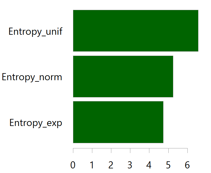
As expected a uniform random variable has is measured to have more randomness in it, than a normal or exponential random variables. The log operator makes the ranking, but it also makes the difference hard to evaluate due to the non-linearity.
Perhaps the most well known measure building on Shannon’s entropy formula is the Kullback – Leibler Divergence, which also give the “where”, and not only the “how much”.
Information theory clashes with robust statistics
It occurred to me that in robust statistics we usually downweight those observations which are flagged as outliers. They are flagged as outliers since they don’t appear often. However, looking at the only formula on this page, those observations would actually signify the highest additional informational value!
Makes sense really, if you only have a couple of flash-crashes to study then you better study them well, rather than removing\downweighting them on account that they don’t belong with the distribution. robust statistics: -1, information theory: +1.
Reference
Information Theory, Inference and Learning Algorithms


