PCA as regression

In a previous post on this subject, we related the loadings of the principal components (PC’s) from the singular value decomposition (SVD) to regression coefficients of the PC’s onto the X matrix. This is normal given the fact that the factors are supposed to condense the information in X, and what better way to do that than to minimize the sum of squares between a linear combination of X (the factors) to the X matrix itself. A reader was asking where does principal component regression (PCR) enter. Here we relate the PCR to the usual OLS.

First and quickly, Singular Value Decomposition (SVD) of X gives us

$X = UDV^{T},$

which also uncomfortably relaxes whatever intuition we managed to hold onto thus far. We plow through nonetheless. Take it as a given that if the X is scaled, then the OLS coefficients can be expressed as

$\beta_{ols} = V D^{-1} U^T y = \sum_{i=1}^p \frac{u_i^{T}y }{\sigma_i} v_i,$

where $p$ is the number of columns in X, the $\sigma_i$ is the $ith$ singular value (arranged is descending order), $u_i$ is the $ith$ left singular vectors of X and $v_i$ is the $ith$ right singular vectors of X. The equation is called the expansion of $\beta_{ols}$ in terms of the right singular vectors of X. In order for to put this mambo-jambo to work lets use the same code from previous post. We create a Y variable which will be the returns of the SPY ETF, and the X matrix will be the returns of the one day lagged ETF’s: IEF, TLT, SPY, QQQ.


# We start with the same code given in the previous post:
library(quantmod)
sym = c('IEF','TLT','SPY','QQQ')
l=length(sym)
end<-format(as.Date("2016-01-01"), "%Y-%m-%d")
start<-format(as.Date("2007-01-01"), "%Y-%m-%d")
dat0 = (getSymbols(sym[4], src="google", from=start, to=end, auto.assign = F))
n = NROW(dat0)
dat = array(dim = c(n, NCOL(dat0),l)) ; prlev = matrix(nrow = n, ncol = l)
for (i in 1:l){
 dat0 = (getSymbols(sym[i], src="google", from=start, to=end, auto.assign = F))
 dat[1:length(dat0[,i]),,i] = dat0 
# Average Price during the day
  prlev[1:NROW(dat[,,i]),i] = as.numeric(dat[,4,i]+dat[,1,i]+dat[,2,i]+dat[,3,i])/4
}
time <- index(dat0)
x <- na.omit(prlev) # omit about 20 missings
TT <- NROW(x)
y <- x[2:NROW(x), 3] - x[1:(NROW(x)-1), 3] # the return on the SPY
x <- cbind(rep(1,(TT-1)), x[1:(TT-1),]) # add intercept 
p <- NCOL(x)
lm0 <- lm(y ~  0 + x )

## now replicate the math above:
# in matrix form:
svd_x <- svd(x)
beta_ols <- svd_x$v  %*% solve(diag(svd_x$d)) %*% t(svd_x$u) %*%y
# in vector form:
beta_ols_vector <- matrix(nrow = 5, ncol = 5)
for ( i in 1:5){ 
 beta_ols_vector[,i] <- t(svd_x$u[,i])%*%y * 1/(svd_x$d[i]) * svd_x$v[,i] # sum of p vectors of length p
}
beta_ols_vector <- apply(beta_ols_vector, 1, sum)
# results:
> cat(beta_ols_vector)
-2.92 0.0548 -0.0235 0.00601 -0.0124
> cat(beta_ols)
-2.92 0.0548 -0.0235 0.00601 -0.0124
> cat(summary(lm0)$coef[,1])
-2.92 0.0548 -0.0235 0.00601 -0.0124

# We start with the same code given in the previous post:

library(quantmod)

sym = c('IEF','TLT','SPY','QQQ')

l=length(sym)

end<-format(as.Date("2016-01-01"), "%Y-%m-%d")

start<-format(as.Date("2007-01-01"), "%Y-%m-%d")

dat0 = (getSymbols(sym[4], src="google", from=start, to=end, auto.assign = F))

n = NROW(dat0)

dat = array(dim = c(n, NCOL(dat0),l)) ; prlev = matrix(nrow = n, ncol = l)

for (i in 1:l){

dat0 = (getSymbols(sym[i], src="google", from=start, to=end, auto.assign = F))

dat[1:length(dat0[,i]),,i] = dat0

# Average Price during the day

prlev[1:NROW(dat[,,i]),i] = as.numeric(dat[,4,i]+dat[,1,i]+dat[,2,i]+dat[,3,i])/4

}

time <- index(dat0)

x <- na.omit(prlev) # omit about 20 missings

TT <- NROW(x)

y <- x[2:NROW(x), 3] - x[1:(NROW(x)-1), 3] # the return on the SPY

x <- cbind(rep(1,(TT-1)), x[1:(TT-1),]) # add intercept

p <- NCOL(x)

lm0 <- lm(y ~ 0 + x )

## now replicate the math above:

# in matrix form:

svd_x <- svd(x)

beta_ols <- svd_x$v %*% solve(diag(svd_x$d)) %*% t(svd_x$u) %*%y

# in vector form:

beta_ols_vector <- matrix(nrow = 5, ncol = 5)

for ( i in 1:5){

beta_ols_vector[,i] <- t(svd_x$u[,i])%*%y * 1/(svd_x$d[i]) * svd_x$v[,i] # sum of p vectors of length p

}

beta_ols_vector <- apply(beta_ols_vector, 1, sum)

# results:

> cat(beta_ols_vector)

-2.92 0.0548 -0.0235 0.00601 -0.0124

> cat(beta_ols)

-2.92 0.0548 -0.0235 0.00601 -0.0124

> cat(summary(lm0)$coef[,1])

-2.92 0.0548 -0.0235 0.00601 -0.0124

Great. Now, the big advantage of PCR is the dimension reduction. In the usual regression, if dimension reduction is what we are after, why not simply drop the few columns from X, but which goddammit? Enter PCR, we rotate the X matrix and construct factors, such that most of the information is captured in the first few factors. Then, we drop the rest of the factors that do not contribute much. We can simply drop them from the regression without concerning ourselves with changes in the other coefficients due to correlation, as correlation between the factors is zero by construction, say they are orthogonal if you want to sound important. Once the factors are created, simply regress the dependent variable on the, say $m$ chosen number of factors (more on number of factors in a sec), and behold that we can express the coefficients of the PCR in terms of the original X (granted, the SVD of X):

$\beta_{PCR} = D^{-1} U^T y = \sum_{i=1}^m \frac{u_i^{T}y }{\sigma_i} v_i.$

We just drop the left singular vector.


pc <- prcomp(x, center= F)
factors <- pc$x
pcr <-lm(y ~ 0 + factors)
beta_pcr <- solve(diag(svd_x$d)) %*% t(svd_x$u) %*% y
cat((summary(pcr)$coef[,1]))
cat(t(beta_pcr))
# results:
> cat((summary(pcr)$coef[,1]))
0.00014 0.000743 -0.00364 -0.0195 2.92
> cat(t(beta_pcr))
0.00014 0.000743 -0.00364 -0.0195 2.92

pc <- prcomp(x, center= F)

factors <- pc$x

pcr <-lm(y ~ 0 + factors)

beta_pcr <- solve(diag(svd_x$d)) %*% t(svd_x$u) %*% y

cat((summary(pcr)$coef[,1]))

cat(t(beta_pcr))

# results:

> cat((summary(pcr)$coef[,1]))

0.00014 0.000743 -0.00364 -0.0195 2.92

> cat(t(beta_pcr))

0.00014 0.000743 -0.00364 -0.0195 2.92

We don’t need to use all factors. There is ample research, dating way back, in regards to the correct number of factors. This is theoretically very interesting, I am not saying, but practically no one will condemn you for simply eyeballing the percent of variance explained plot. More often than not, it is quite indicative and provides a good sense as to the number of factors that capture most of the embedded information in X.

As an aside, if we have a completely random matrix, each factor should carry equal weight. This is the starting point of most of the research that went, and still going, into this area. Here is the variance explained of our data and how it should look like it the matrix is completely random:


barplot(summary(pc)$importance[2,])
title("Variance explained by the factors, from first (most left)  to fifth (most right)", 
      sub= "our data")
temp <- matrix(ncol=5,nrow=100)
for( i in 1:5){
 temp[,i] <- rnorm(100)
}
pc_random <- prcomp(temp)
barplot(summary(pc_random)$importance[2,])
title("Variance explained by the factors, from first (most left)  to fifth (most right)", 
      sub= "random data, no factor structure")

barplot(summary(pc)$importance[2,])

title("Variance explained by the factors, from first (most left) to fifth (most right)",

sub= "our data")

temp <- matrix(ncol=5,nrow=100)

for( i in 1:5){

temp[,i] <- rnorm(100)

}

pc_random <- prcomp(temp)

barplot(summary(pc_random)$importance[2,])

title("Variance explained by the factors, from first (most left) to fifth (most right)",

sub= "random data, no factor structure")

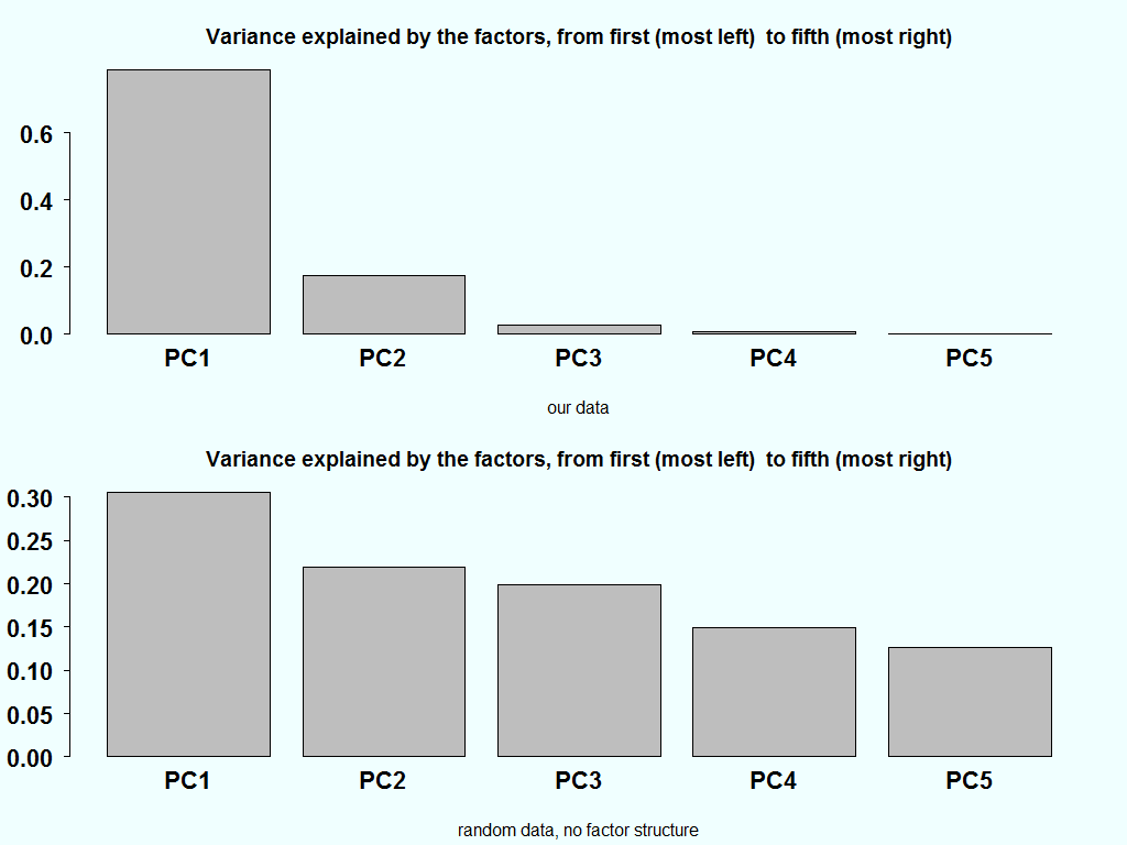
The variance explained in the bottom chart, ideally should be equal. But since there is also estimation noise in the estimation of the eigenvalue, combined with the fact that they are ordered in a descendent order, creates the downwards slant in the bottom bar plot.

Related book:

You might also like:

PCA as regression (2)

You might also like:

One comment on “PCA as regression (2)”

Leave a Reply