What is the Kernel Trick?

Every so often I read about the kernel trick. Each time I read about it I need to relearn what it is. Now I am thinking “Eran, don’t you have this fancy blog of yours where you write about statistics you don’t want to forget?” and then: “why indeed I do have a fancy blog where I write about statistics I don’t want to forget”. So in this post I explain the “trick” in kernel trick and why it is useful.

Why do we need the kernel trick anyway?

The kernel trick is helpful for expanding any data from its original dimension to higher dimension. Fine, who cares?. Well, in life we often benefit from dimension expansion. Higher dimension makes for a richer data representation, which statistical models can exploit to create better predictions. Let’s look at a textbook example.

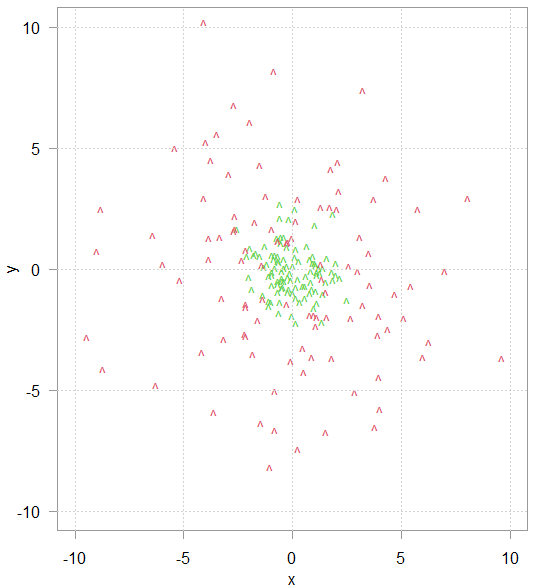
Consider this toy data in figure 1. The task is to classify the green and red data points based on their (x,y) coordinates. Logistic regression, or any other model with linear decision boundary will not do, because the data is not linearly separable.

But if we add another variable – the sum of the squared variables: x² + y² then the new richer data representation is now better linearly separated, as can be seen in the plot below (rotate for a better view).
<br />
The new variable ( $x^2 + y^2$ ) “pulls” the high value points up along the third axis keeping the inner class “on the ground” so to speak. Now if a new data point arrives, it will be easier to classify it, even by using “just” a logistic regression with those three coordinates as explanatory variables. This is why it is often (but not always) beneficial to add higher order terms. Forward to talk about the trick.

In what way the kernel trick is helpful?

After we have seen that it can be beneficial to add higher order terms (and\or interactions between the variables) we now show how to create those, “manually”. After which we will apply the kernel trick. Consider we only have two observations x1 and x2, with three variables each:
x1 <- c(3,4,5) x2 <- c(1,2,4)
We would like to add the squares and interactions between the variables:
const <- sqrt(2) # ignore this for now a <- x1^2 b <- x2^2 # interaction between 2 and 1: c1 <- const*x1[2]*x1[1] # interaction between 3 and 1: c2 <- const*x1[3]*x1[1] # etc. etc. c3 <- const*x1[3]*x1[2]

c4 <- const*x2[2]*x2[1] c5 <- const*x2[3]*x2[1] c6 <- const*x2[3]*x2[2]
Many models need the calculation dot product (think how often you see $X ^{\prime} X$ ), support vector machines (SVM) in particular. In our code we now have 4 terms for each of our observations:
c(a, c1, c2, c3) %*% c(b, c4, c5, c6) # 961
The c(a, c1, c2, c3) corresponds to what you sometimes see in text book as $\Phi(x)$ , which means a function applied to x to expand it to (in this example) its square and interactions:

$\begin{array}{l} \phi(\mathbf{x1})=\left(x1_{1}^{2}, x1_{1} x1_{2}, x1_{1} x1_{3}, x1_{2} x1_{1}, x1_{2}^{2}, x1_{2} x1_{3}, x1_{3} x1_{1}, x1_{3} x1_{2}, x1_{3}^{2}\right)^{T} \\ \phi(\mathbf{x2})=\left(x2_{1}^{2}, x2_{1} x2_{2}, x2_{1} x2_{3}, x2_{2} x2_{1}, x2_{2}^{2}, x2_{2} x2_{3}, x2_{3} x2_{1}, x2_{3} x2_{2}, x2_{3}^{2}\right)^{T} \end{array}$

Note that we use we consider z1*z2 to be the same as z2*z1. That is the reason for the line const <- sqrt(2) at the beginning of the code.

Using the kernel trick we can spare the individual computation and go directly to the end result by simply first dot-product the variables in their original space, and only then applying the kernel function. In this case the kernel function is $k(\mathbf{z1}, \mathbf{z2})= \left(\mathbf{z1}^{T} \mathbf{z2}\right)^{2}$ so simply taking the dot-product and square it. Like so:
(x1[1:3]%*%x2[1:3])^2 # 961

As you can see the result is the same, and the "trick" refers to the fact that we elegantly leaped over the computation of the individual terms, and found a function which returns the same result, as if we have, in fact, computed the exact expansion (which we didn't). Effectively we have reduced computational complexity from an exponential growth of O(#variables^2) to a linear growth of O(#variables). This reduction in computational complexity paves the way to higher dimensional representation, which would otherwise be computationally prohibitive. That said, I think a kernel tip would be a better dubbing, the word "trick" makes it sounds like it's more than it is.

Can I do this trick with any function?

No. Mercer’s theorem of functional analysis tells us this trick only works with continuous functions that are positive everywhere. See the paper "Nonlinear component analysis as a kernel eigenvalue problem" (particularly Appendix C) in the reference for a readable exposition. That is why we have few kernel functions, not too many, used by everyone. The library kernlab in R and the module sklearn.metrics.pairwise has everything you need for computation. The same computation we did "manually" above could also be done using the built-in functions:


> polykernel <- polydot(degree = 2, scale = 1, offset = 0)
> polykernel(x1, x2) 
     [,1]
[1,]  961

> polykernel <- polydot(degree = 2, scale = 1, offset = 0)

> polykernel(x1, x2)

[,1]

[1,] 961

References

Learning with Kernels: Support Vector Machines

Schölkopf, Bernhard, Alexander Smola, and Klaus-Robert Müller. "Nonlinear component analysis as a kernel eigenvalue problem." Neural computation 10, no. 5 (1998): 1299-1319.