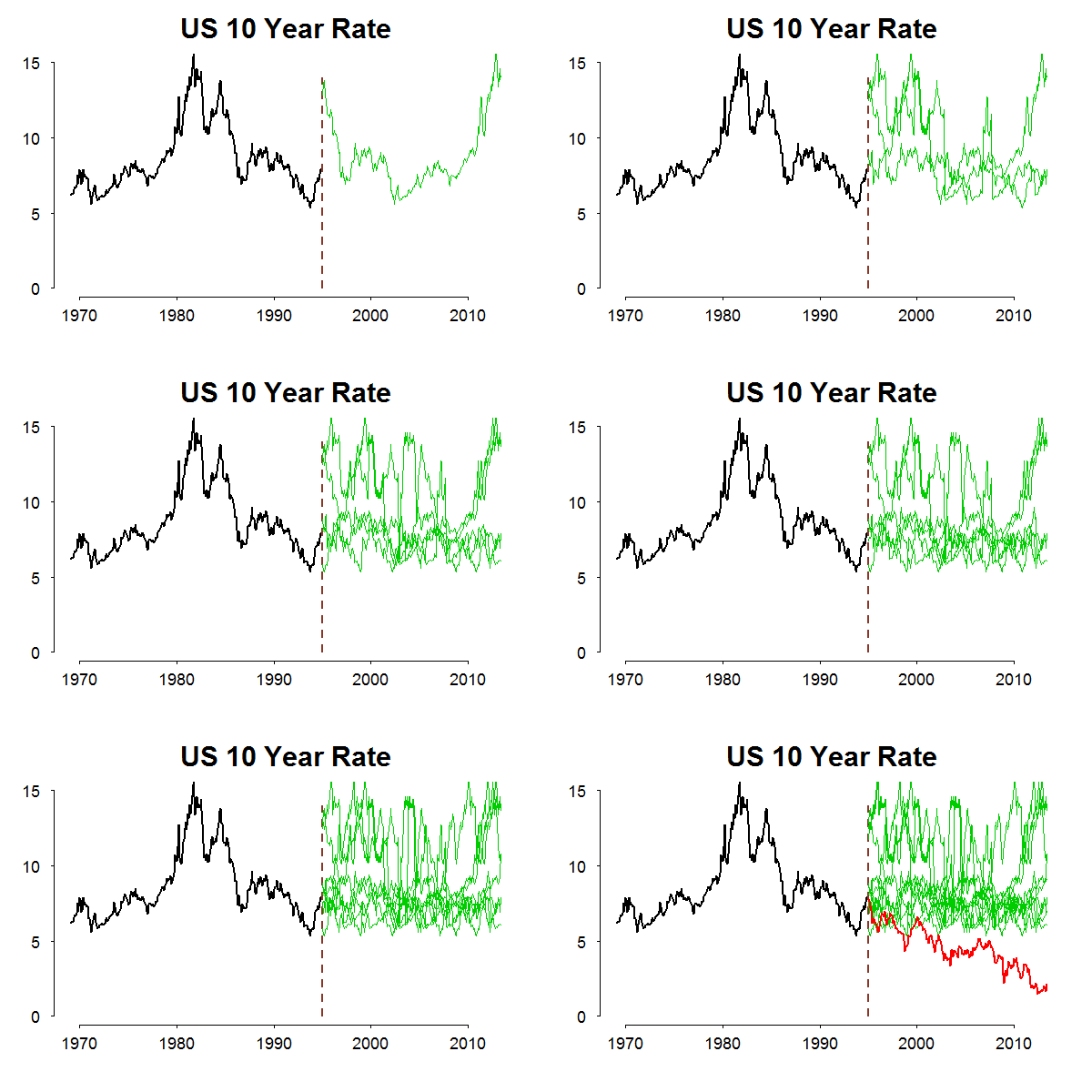
The title reads Bootstrap criticism, but in fact it should be Non-parametric bootstrap criticism. I am all in favour of Bootstrapping, but I point here to a major drawback.
The point is that we will never reach a scenario which is not covered by observed past. In most cases, we have enough past (or a wide range of observations) so that we feel comfortable, but not always. As an example, the Eurozone is only around for a decade or so in current configuration. Another example, if today it is 1995, and we think about possible futures for the interest rate series, non-parametric bootstrap which heavily relies on the data, a good thing in general (the frequenist in me talking), is a limited tool for the job. The following animation shows possible “futures” for the rate series in green and the red line is the actual realization.
 As you can see, in the sample we have the series did not travel to the low interest rates environment observed today. Therefore, we have no chance to include this area in our set of possibilities (or, in probability jargon, to extend our support, to extend Omega). The big plus of non-parametric bootstrap is that it is strictly data-based, without any distributional assumption, the big minus is the same, it is strictly data-based. This disadvantage can be worked around by adding more assumptions and simulate from some distribution, a known one or a one you create for yourself given your own subjective guess.
Thinking ahead, we have never observed negative nominal interest rates, for a good economic reason, but you never know what policy makers may want to do to encourage consumption :), fingers crossed.
Code for the animation:
|
1 2 3 4 5 6 7 8 9 10 11 12 13 14 15 16 17 |
df = data.frame(Time,Rate) # that is the data frame TT = NROW(df) cpoint= which(df$Time=="1994-12-31") saveGIF({ par(mfrow=c(1,1),bty = "n") for (m in 1:10){ plot(c(df$Rate[1:cpoint], rep(NA,TT-cpoint))~df$Time, ylim = c(0,15),ty = "l", ylab = "", tck = -0.01, xlab = " ",cex=2.8,main = "US 10 Year Rate", cex.lab = 1.5,cex.main = 2.5, lwd=2.5, las = 1,cex.axis = 1.3) segments(x0=df$Time[cpoint],y0=0,x1=df$Time[cpoint],y1=14, col='brown',lwd=2.5,lty=2) for (k in 1:m){ lines(ystar[1:length(df$Time[cpoint]),k]~df$Time[cpoint],col = 3) }} # code for creating ystar is give in https://eranraviv.com/blog/bootstrapping-time-series-r-code/ points(df$Rate[cpoint:(TT)]~df$Time[cpoint],col = 2,ty ="l",lwd=lwd1) } # You need to install ImageMagic to animate the plot |


Hi,
Nice example showing that not everything should be entirely data-driven. Models and priors are and will always be useful.
I am not sure how you did your bootstrapping (didn’t examine the code closely), but usually one first-differences the time series and bootstraps using reshuffled differences, in my experience.
Thanks for the comment. You raise a good point, the code I use is suited for weakly dependent time series while the rates are clearly very strongly dependent. I thought a bit about your suggestion to difference the series and then bootstrap. This would result in many bootstrapped series which reach unreasonable values (e.g. -6% nominal rate). Perhaps there is a work-around to that but the criticism is general. Think 06/05/2010 during the flash crash, you will never get such a crash from bootstrapping prior to that specific date (at least not using non-parametric bootstrap).