Bootstrap example

Bootstrap your way into robust inference. Wow, that was fun to write..

Introduction
Say you made a simple regression, now you have your . You wish to know if it is significantly different from (say) zero. In general, people look at the statistic or p.value reported by their software of choice, (heRe). Thing is, this p.value calculation relies on the distribution of your dependent variable. Your software assumes normal distribution if not told differently, how so? for example, the (95%) confidence interval is , the 1.96 comes from the normal distribution.
It is advisable not to do that, the beauty in bootstrapping* is that it is distribution untroubled, it’s valid for dependent which is Gaussian, Cauchy, or whatever. You can defend yourself against misspecification, and\or use the tool for inference when the underlying distribution is unknown.

I was not here 40 years ago but they say calculations were slow back then, not any more, take advantage of your Dell or your “meant for you” MacBook. We will see that it is better to add the non in the nonparametric, specifically in financial context, but that holds in general. You can still keep your distribution assumption but at least have a look at what happens when you relax it. The way to do that is by using bootstrap, the idea is intuitive and simple.

The idea
John Fox wrote: “The population is to the sample as the sample is to the bootstrap samples”.. Tadaaam.. but what does this mean?  your estimate of which came from the sample, is suppose to estimate the “real” , the population  , which is unknown. Now take a sample from the sample, we call that sample a bootstrap sample, estimate your according to this (bootstrap)sample, now this new estimate is an estimate for your original , the one coming from the original data. For clarity, say you have 3 observations, first is {x = 0.7,y = 0.6}, second is {whatever}, third is {whatever}, now, an example of sample from the sample would be the shuffled ordering: first is {whatever}, second is {x = 0.7,y = 0.6}, third is {whatever}. This “shuffling” is what we call the bootstrap sample, note that any observation can be chosen more than once or not at all, that is, we sample with replacement. Now we estimate the same statistic (in our case ) again.
Repeat this sample and estimate many times, you have many bootstrapped estimates, now you can check how do these guys behave. One thing you can do with it is to bootstrap confidence intervals (CI) for your estimate, without the need for underlying distributional assumption.

In R
In R, “boot” package will do the trick:

You can zoom in on which indices were picked at each bootstrap take, what was the exact permutation, you do that using the function boot.array:

More transparent
You can better understand it if you can code it yourself, for a simple problem like bootstrapping confidence intervals it is even simpler and faster:

How bad are your current confidence interval?
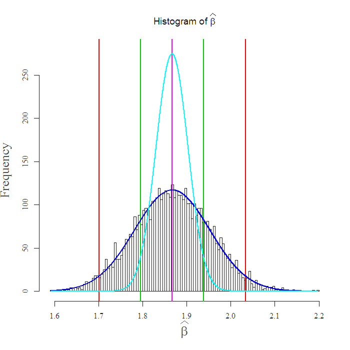
Does it really matter? maybe it’s not worth the trouble. As an illustration I use stock returns which are known to have fat tails, meaning more observations far from the center. Take a look at the following figure:

That is the Morgan Stanley with the market. The estimate is centered at 1.87. The green vertical lines are the (95%) confidence interval reported by the the “lm” function, the red vertical lines are the equivalent nonparametric confidence intervals, the light blue curve is the normal density.

Notice how different is the interval from the nonparametric bootstrap, which is more accurate in this case. For example, it may be that the parameter is actually 2, you can see the software output rejects this possibility since it assumes normality, yet the bootstrap confidence interval indeed covers the value 2. So, an investor who thinks that “in my portfolio all beta’s are smaller than 2 with a 95% CI” is mistaken to hold Morgan Stanley as such. This check takes about 80 seconds, so I would think twice before plugging it in a double “for” loop. However, if you are social scientist or similar, beef up your standard (normal) output with this robust analysis.
Wrap up
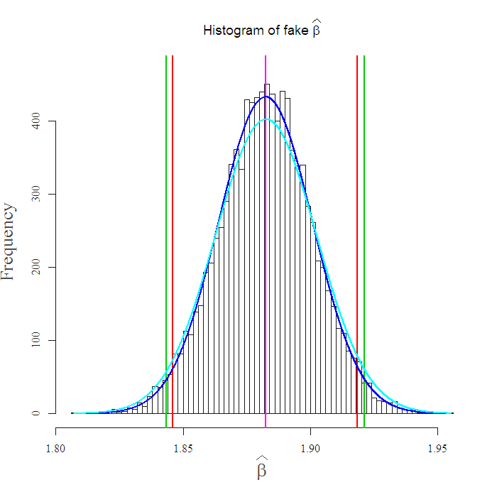
Here you can see that when you use the bootstrapped confidence interval, when the normal distribution assumption IS valid, you are not that worse off (though you will need to wait these 80 seconds nontheless 🙂 ). I created a fake normal return distribution using same center and standard deviation as reported, and made the exact same analysis:

Again, I simulated from a normal distribution using same center and standard deviation as reported by the “lm”, you can see that the intervals are close to each other which concludes this post, using the parametric confidence interval, from the assumed normal distribution is in some sense suboptimal, since you don’t lose much even if it IS normal.
You can see the remaining code and some references below. Thanks for reading.

Comments
* Naturally we only cover the idea here, there is lots of bootstrapping literature, we only tasted nonparametric bootstrap.

Related literature
[asa onelinertpl]0521574714[/asa]
[asa onelinertpl]0412042312[/asa]
[asa onelinertpl]0817643869[/asa]