More good news for the statistical bootstrap. A new paper in the prestigious Econometrica journal makes two interesting points.
The first point made in the “Bootstrap Standard Error Estimates and Inference” emphasizes is that the bootstrap is actually based on weak convergence. Weak convergence does not imply convergence of moments. Researchers usually ignore that fact and use the bootstrap second moment as an estimate nonetheless.
Using the bootstrap standard deviation as a plug-in estimate is a common mistake, why? For the special case of the mean it’s not a mistake, so perhaps people presumed that if it’s good for the mean, it’s good for other statistics as well (but it is not). More importantly, it’s an easy mistake to make because it’s so straightforward to do. The second point the authors make is to prove that if you use an estimate based on the second moment of the bootstrap, you are being overly conservative.
Illustrative Example
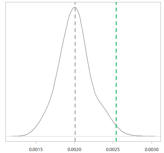
To illustrate this mistake that we are talking about – using the bootstrap standard deviation as a stand-in for the real standard deviation – consider the median as our statistic of interest; in this special case of the median wikipedia tells us what is the asymptotic variance of the estimate. This following figure shows the asymptotic variance versus using the bootstrap variance as an estimate (I use the median of exponential distribution, replication code for the figure in the end of this post). The dashed green line is the bootstrap estimate, while the density shows the distribution of the asymptotic variance of the estimate. You can see that the bootstrap estimate is on the high side.
The bootstrap estimate for the standard deviation is too high
Why should we consider this to be good news for the bootstrap? I am happy you ask.
For all inference which relied wrongly on the bootstrap standard deviation there are two options: (1) Rejection of the null hypothesis, or (2) a failure to reject the null hypothesis. The Econometrica paper shows an overestimate of the variance estimate based on the bootstrap, which means a rejection is harder to achieve. So all those hypotheses that were rejected are nonetheless certified, since going back and correcting the mistake will make it even easier to reject. Those researchers who failed to reject now have a chance for a test-retake, knowing that their inference was overly conservative. Personally speaking, it is easy to use the bootstrap standard deviation as an estimate, so I think I will simply keep doing that, even though I know I am theoretically wrong. Next time I will need inference I would not mind knowing that I am being overly conservative. In my opinion it’s a cheap price to pay for the bootstrap computational convenience. Good.
Code
|
1 2 3 4 5 6 7 8 9 10 11 12 13 14 15 16 17 18 19 20 |
library(magrittr) TT <- 500 ratee <- 1 x <- rexp(TT, rate= ratee) # bootstrap rr <- 1000 boot_mat <- matrix(ncol= rr, nrow= TT) for (i in seq_len(rr)){ boot_mat[,i] <- sample(x, replace= T) } boot_med <- apply(boot_mat, 2, median) density(boot_med) %>% plot abline(v = log(2)/ratee, lty= "dashed", lwd=3) boot_med %>% var Asym_var <- 1/(4*TT*(ratee*exp(-ratee*boot_med))^2 ) density(Asym_var, adjust = 3) %>% plot(main="", ylab="", yaxt= "n", lwd=2) abline(v = var(boot_med), lty= "dashed", lwd=3, col= "green") abline(v = mean(Asym_var), lty= "dashed", lwd=3) |


Dear Mr. Raviv,
thank you for this interesting post. I tried to replicate your analysis in R. However, the code can not run as you use a symbol/constant “e_col” which is not defined. Could it be that I have to load a specfic package? For the pipe operator I would load tidyverse. Do I need anything in addition?
Another thing:
– You use log(2)/ratee – this is the anlytic formula for the median, right?
– Could you please give a short remark about the formula 1/(4*TT*(ratee*exp(-ratee*boot_med))^2 ).
Thank you and kind regards,
Richard Warnung
Thanks for the comment. Code is now updated, loading the
magrittr. e_col is my own-defined color, just change that to whichever color you want.“You use log(2)/ratee – this is the anlytic formula for the median, right?” right.
“Could you please give a short remark about the formula 1/(4*TT*(ratee*exp(-ratee*boot_med))^2 ).” See here for the corresponding variance of the sample median.
Thank you for these clarifications! Also, thank you for communicating these results. This will turn out very useful when we need to justify conclusions from bootstrap analyses!
Hi Eran,
I might be doing something wrong or not getting the idea fully but when i try to execute repeatedly provided R code i get bootstrap estimates (green line) that are on the down side of the asymptotic variance. Do you get same result in repeated executions of the code?
Thank you,
Ivan
Re above comment, wanted to clarify that in general bootstrap estimates (green line) are on the high side of the asymptotic variance in repeated executions of the code but on some occasions results appear on down side as well.