On Central Moments

Sometimes I read academic literature, and often times those papers contain some proofs. I usually gloss over some innocent-looking assumptions on moments’ existence, invariably popping before derivations of theorems or lemmas. Here is one among countless examples, actually taken from Making and Evaluating Point Forecasts: 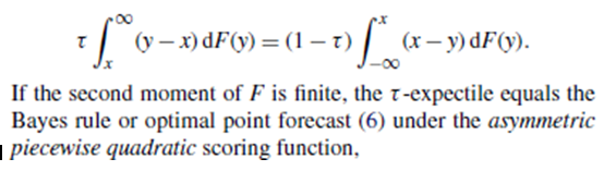“If the second moment is finite…”, the term “moment” crept into the statistical literature from physics, and earlier than that from mechanics. How exactly I could not figure out. The term “moment” refers to the average (or expected) distance from some point. If that point is the expectation (rather than zero), then we say the moment is a central moment. The distance can also be squared, or it can be in the power of 3, or in the power of a general k. Thus first order moment about mean is always zero (the raw first moment, which is about zero is the mean). The second order moment about the mean gives us the variance. The third order moment about the mean gives us the skewness and so on.

The notion of existence of moments is hard to comprehend, perhaps not as hard to comprehend as how the infinite series whose terms are the natural numbers sum up to -1/12, but still mind boggling. The reason for the difficulty is clear, we occupy our day-to-day, not the metaphysical. In real-life, we have samples, and I bet you have yet to encounter the sample which has infinite standard deviation.

Formal definition of central moments

Formally speaking, a central population moment of a random variable X is defined as:

(1)  

Equation (1) is theoretical. In real life most data do not even follow a well defined distribution, like one of those nicely behaved exponential family set of probability distributions.

We always and only compute the central sample moments

(2)  

Those term in equation (2) are estimates of those terms in equation (1). Excluding complicated Multimodal distributions, if we estimate well the first four moments (raw first moment: mean, central moments of order 2,3 and 4: variance skewness and kurtosis) those four give a good description of how the distribution looks like. So writing them down in a table format can replace a density or a histogram figure without much loss of information.

Simulation

We can call simulation to our aid in order to understand the difficult concept of existence of central moments. The concept has much to do with extreme value theory and heavy tail behavior. We can simulate from a distribution for which we know some moments are not defined properly and have a look at it.

One textbook example for a distribution like that is the Cauchy distribution. We saw the Cauchy distribution before, when discussing heavy tails in the past. Heavy tails means extreme values with non-negligible probability, which is precisely why central moments are not defined, because they never stabilize, because of the non-negligible probability of a large deviation. To see this clearly, pretend that you have a process which follows the Cauchy distribution. You are interested in the determination of the second moment, the theoretical standard deviation of the process (k=2 in equation (1) above). You try to estimate this quantity using its empirical counterpart. So with each new observation you compute the standard deviation based on all the observation you have so far, waiting for your estimate to settle. Don’t hold your breath. It does not.

Have a look:

You can see how the estimate of the standard deviation is about to converge to some value after around 5000 draws, but very large observations arrive and mess up the convergence.

We can do the same exercise for another distribution for which we know the second moment is well defined:

What we see in the second figure is the same computation, though now the process follows a standard normal distribution. You can see how the computation of the standard deviation is stabilized as the process continues.

Remember, the support of the Normal distribution is the same as that of the Cauchy distribution, but for Normal distribution the probability of extreme values is negligible. The probability of large deviations from the mean is too small to trouble the convergence.

Another side-insight you get from this exercise is: you can see what they mean when people use colloquial term ‘Burn-in period’ which is oftentimes heard when dealing with Markov chain Monte Carlo (MCMC)computation. If we start the computation of the standard deviation too early, it takes much longer to converge to the real standard deviation of one. So we can (should?) get rid of the first part, which is quite wiggly and interrupting. We will see much faster convergence towards the actual value of the standard deviation (which is 1) if we burn that wiggly part.

Without the aid of computers, past statistical giants were forced to imagine those, or similar figures, using thought experiments only. I wonder what thought experiments needed nowadays, when we can do so much even with only a laptop.

Stock data

Finally, let’s now examine the result of this same exercise using stock data. I pull data from 2006 for the SPY ticker, and compute the estimate for the standard deviation using expanding window:

Notice the similarity of this figure to that from the Cauchy distribution. During the global financial crisis we have seen pretty unusual deviations from the mean, those were strong enough to rattle the series and interrupt convergence. This is the same heavy tail story told from a different angle. The angle of non-existent standard deviation.