Most profitable hedge fund style

This is not an investment advice!!

Couple of weeks back, during amst-R-dam user group talk on backtesting trading strategies using R, I mentioned the most effective style for hedge funds is relative value statistical arbitrage, I read it somewhere. After the talk was over, I was not sure anymore if it was correct to say it and decided to check it.

Will be interesting to know what is an effective ~~profitable~~ investment style. Say you face two similar hedge funds, clashing only with their investment style. The one is emerging markets expert, busy collecting its coupons there. The other is event-driven, fishing mergers or hostile takeovers for opportunities. Both pitchers look alike, even same tie pattern, which style is more likely to yield better? In addition, there are also products that track performance of hedge funds index according to style, so you can get the exposure to a style without really being engaged in the strategy itself. You don’t have to be an emerging market expert to get emerging market investment style, just invest in the index that tracks this style, oh yeah, remember that past performance is no indication of future results, #$% covering at its best.

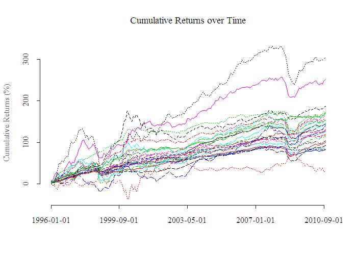
Data is taken from here (registration needed). As an example of a style, “Special Situations” style fund primarily focuses on opportunities in equity related instruments of companies currently engaged in a corporate transaction, security issuance/repurchase, asset sales and alike. Our universe includes all kind of styles, 27 in total, which you can review in the Appendix. What interests us is which of these styles performs best, or more accurately, has the best risk reward ratio. Our time span is from January 96 until October 2010, monthly returns. For the feel of the data, here is a small figure of the cumulative returns of the different styles:The top black style looks promising, but returns are only part of the game, we need a more intelligent performance measure, risk adjusted. We use Sharp Ratio, Omega Ratio and Sortino Ratio, Appendix for details. The top two lines, the pink (Equity Hedged Sector Energy and Basic Materials) and the black (Emerging Markets Russia and Eastern Europe), despite their high cumulative return, do not turn up to be very effective styles, probably due to the sharp draw-downs during 2008-2009.
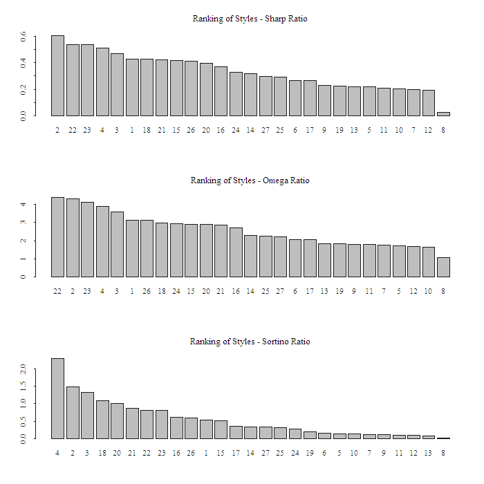
Here are the results:

Ranking of Investment Styles — In the appendix you can see the styles that match the numbers

The names of the styles were too long to be incorporated in the graph, but you can match them with the list in the Appendix. The first two measures, the Sharp Ratio and the Omega Ratio are highly correlated, the Sortino Ratio measure less. Style number 8 (Equity Hedge Short Bias) is top loser in all categories. Style number 2 (Event Driven Merger Arbitrage) is a strong one.

Here is a more concise list according to Sharp Ratio measure:

	Winners	Losers
1	ED..Merger.Arbitrage	EH..Short.Bias
2	Relative.Value..Total.	Emerging.Markets..Latin.America
3	RV..Fixed.Income.Asset.	EH..Sector…Technology.Healthcare

What are the winners doing?

Merger Arbitrage strategies employ an investment process primarily focused on companies which are currently engaged in a corporate transaction. So two companies that are about to merge for example, you can sell the high and buy the low, they are expected to become one soon, so you can collect the spread.

Two and three are Relative Value: Investment style which compares securities that have close relation to each other, when one is mispriced relative to the other, you short the one which is “expensive” and long the “cheap one” expecting convergence in the future. “Total”, (in row 2) probably refers to full flexibility and “Fixed.Income.Asset” refers to sub category of only fixed income investments. So, all in all, I feel comfortable with my statement at the talk. Relative value emerges as a winning style. Which style should you try to avoid?

Short-Biased strategies employ analytical techniques in which the investment thesis is predicated on assessment of the valuation characteristics on the underlying companies with the goal of identifying overvalued companies. I wrote about this kind of trials long ago here. Nice to see this result. Thanks for reading, as always code is below:
Appendix
the universe is:

	Strategy
1	ED..Distressed.Restructuring
2	ED..Merger.Arbitrage
3	ED..Private.Issue.Regulation.D
4	EH..Equity.Market.Neutral
5	EH..Quantitative.Direc
6	EH..Sector…Energy.Basic.Materials
7	EH..Sector…Technology.Healthcare
8	EH..Short.Bias
9	Emerging.Markets..Total.
10	Emerging.Markets..Asia.ex.Japan
11	Emerging.Markets..Global
12	Emerging.Markets..Latin.America
13	Emerging.Markets..Russia.Eastern.Europe
14	Equity.Hedge..Total.
15	Event.Driven..Total.
16	FOF..Conservative
17	FOF..Diversified
18	FOF..Market.Defensive
19	FOF..Strategic
20	Macro..Total.
21	Macro..Systematic.Diversified
22	Relative.Value..Total.
23	RV..Fixed.Income.Asset.
24	RV..Fixed.Income.Convertible.Arbitrage
25	RV..Fixed.Income.Corporate
26	RV..Multi.Strategy
27	RV..Yield.Alternatives

FOF = Fund of Funds
EH = Equity Hedge
ED = Event Driven
RV = Relative Value
In case you would like to know what a specific style means check here.
Performance measures:

$Sharp Ratio = \frac{E[R_{style}-R_f]}{\sigma_{style}}$

$OmegaRatio = \frac{\int_{R_{free}}^\infty (1-F(x))\,dx}{\int_{-\infty}^{R_{free}} F(x)dx}$

and in its more intuitive discrete version:

$\frac{ \frac{1}{n} \times \Sigma_{i = 1}^{i = n} Max(R_i - R_{free} ,0) } { \frac{1}{n} \times \Sigma_{i = 1}^{i = n} Max(R_{free} - R_{i} ,0) }$

$Sortino Ratio = \frac{E[R_{style}-R_{free}]}{\sigma^{style}_{DR}}$

where

$\sigma^{style}_{DR} = \sqrt{\Sigma_{i = 1}^{i = n} \frac{min(R_i - R_{free},0)^2 } {n} }$

is what we call downside risk. Since we only compare the styles, we don’t really care about the risk free, as long as it is the same for everyone we can assume without loss of generality that it is zero throughout the analysis.
R code


library(xtable)
x = as.matrix(read.table("hedgefund_dat.txt", sep = "\t",header = T))
x1 = apply(data.matrix(cbind(x[13:length(x[,1]),2:20],x[13:length(x[,1]),27:34])),2,as.numeric) # clean missing
n = length(x1[,1]) # number of obs
style = names(x1[1,]) # store the style
style1 = NULL
for (i in 1:length(style)){ # format the style name
style1[i] = substr(style[i],6,nchar(style[i]))
style1[i] = substr(style1[i],1,nchar(style1[i]) - 6)																			
}								
colnames(x1)<-c(1:dim(x1)[2]) # rename the columns
cum = apply(x1,2,cumsum)
par(mfrow = c(1,1))
time = as.Date(paste("01-",x[13:length(x[,1]),1], sep = ""), "%d-%m-%Y")
head(time,1) ; tail(time,1) # time span
matplot(cum[,13], ty = "l", xaxt = "n", ylab = "Cumulative Returns (%)", main = "Cumulative Returns over Time") 
axis(1,at = seq(1,178,44), time[seq(1,178,44)])
sr = apply(x1,2,mean)/apply(x1,2,sd) # sharp ratio
sor = apply(x1,2,mean)/  # sortino ratio
(apply((apply(x1,2,function(x) ifelse(x<0,x,0))^2),2,sum)/n)
numstyle = NCOL(x1) # number of styles
nomin = NULL ; denom = NULL 
for (i in 1:numstyle){
nomin[i] = sum(ifelse(x1[,i]>0,x1[,i],0))/n
denom[i] = sum(ifelse(x1[,i]<0,x1[,i],0))/n
}
OR = nomin/(-denom) # Omega Ratio
names(OR) <- c(1:27)
names(sor) <- c(1:27)
par(mfrow = c(3,1))
barplot(sr[ rev(order(sr))[1:numstyle] ] , main = "Ranking of Styles - Sharp Ratio")# ,names.arg = style1[rev(order(sr))[1:numstyle]] )
barplot(OR[ rev(order(OR))[1:numstyle] ] , main = "Ranking of Styles - Omega Ratio")
barplot(sor[ rev(order(sor))[1:numstyle] ] , main = "Ranking of Styles - Sortino Ratio")