Spectral Clustering

Some problems are linear, but some problems are non-linear. I presume that you started your education discussing and solving linear problems which is a natural starting point. For non-linear problems solutions often involve an initial processing step. The aim of that initial step is to transform the problem such that it has, again, linear flavor.

A textbook example is the logistic regression, a tried-and-true recipe for getting the best linear boundary between two classes. In a standard neural network model, you will find logistic regression (or multinomial regression for multi-class output) applied on transformed data. Few preceding layers are “devoted” to transform a non-separable input-space into something which linear methods could handle, allowing the logistic regression to solve the problem with relative ease.

The same rationale holds for spectral clustering. Rather than working with the original inputs, work first with a transformed data which would make it easier to solve, and then link back to your original inputs.

Spectral clustering is an important and up-and-coming variant of some fairly standard clustering algorithms. It is a powerful tool to have in your modern statistics tool cabinet. Spectral clustering includes a processing step to help solve non-linear problems, such that they could be solved with those linear algorithms we are so fond of. For example, the undeniably popular K-means.

Contents

Motivation for spectral clustering

“Use a picture. It’s worth a thousand words” (Tess Flanders)

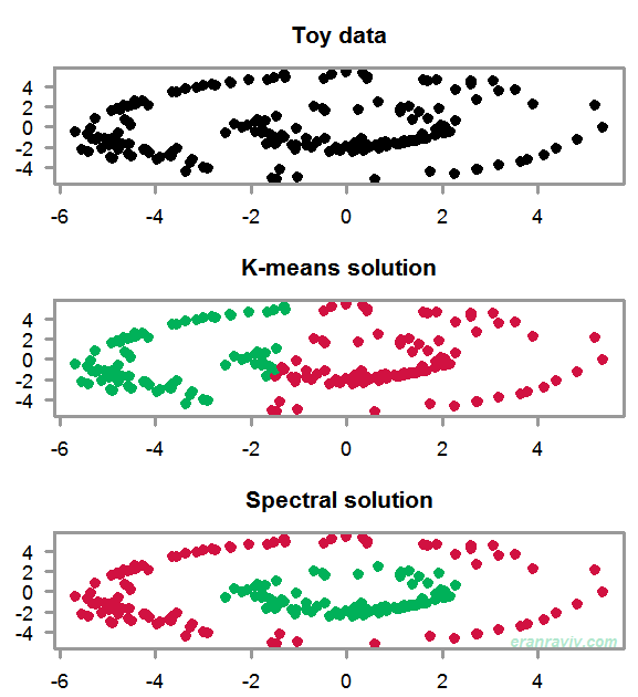
The goal is to create two disjoint clusters. Our toy data has these “two rings” shape to it. You can see that because the data is not linearly separable, the K-means solution does not make much sense. We need to account for the particularly non-linear structure in the data. ~~The way to do that~~ One way to do that is to use the eigensubspace of the data, not even of the data actually, but of a similarity (affinity) matrix of the data. Bit obscure now, but some clarity is en route.

A typical spectral clustering algorithm

Here is the formal algorithm. It is taken from a paper called “On Spectral Clustering” (see references). However, I complement each of the steps with my own explanation for what ~~the hell~~ is going on there. Deep breath, here we go.

Form the affinity matrix $A \in \mathbb{R}^{n \times n} \;$ defined by $A_{i j}=\exp \left(-\left\|s_{i}-s_{j}\right\|^{2} / 2 \sigma^{2}\right)$ if
$i \neq j,$ and $A_{i i}=0$ . We compute the distance between each two points and collect those distances in a matrix. The diagonal is set to zero. The distance here is not something you may be used to, like euclidean for example. But look closely, it has some resemblance. Say you want to quantify similarity rather than distance. One way to do that is to use the inverse. For example, if the distance between two points is ‘tiny'(= $\left\|s_{i}-s_{j}\right\|^{2} / 2 \sigma^{2}$ ), the points $s_i$ and $s_j$ are similar and the quantity $\frac{1}{'tiny'}$ is large, while if the distance between the two point is ‘large’ then similarity should be very small, and so taking the inverse $\frac{1}{'large'}$ would work for us as it would result in a small value. The ugly exponent expression does the same, only instead of taking the inverse we use another function which dictates a more aggressive decay than that of the inverse function; namely $\frac{1}{e^{'distance'}}$ . This function is called Gaussian kerne and is widely used. Now that you understand the idea: moving from distance to similarity in that way, you don’t have to use a Gaussian kernel for your build. As long as you keep in line with the direction: large (small) distance –> small (large) similarity, you can choose some other function which conforms to this story. I have also seen ~~people~~ academics use the t-distribution rather than the Gaussian. In my opinion it needlessly complicates the math. I am doubtful about the added value from tweaking the decay rate around that kernel function, but at the same time perhaps I don’t know enough about this topic.
Define $D$ to be the diagonal matrix whose $(i, i)$ -element is the sum of $A$ ‘s $i$ -th row, and construct the matrix $L=D^{-1 / 2} A D^{-1 / 2}$ . The matrix $L$ is referred to by the somewhat bombastic name: graph Laplacian matrix, not sure where the name comes from. Now, what is the meaning of $D$ ? In graph theory there is a notion of degree. A “too-big-to-fail” bank would have a high degree since a lot of other banks do business with it. In graph theory terms we denote the number of banks connected to that bank $i$ as the degree. Since $A$ is symmetric, you could think about either rows of $A$ or the columns of $A$ . Say our aforementioned bank sits in row number i=4. We sum over all the entries in row $i=4$ , which would mean calculating the strength-of-contentedness of bank $i=4$ with the other banks ( $i \neq 4$ )*. So that is $D$ . Because $D$ is a diagonal matrix, $L$ is a column-scaled and row-scaled version of $A$ (see the Appendix for the formal reason). The matrix $L$ is scaled with the strength-of-contentedness the rows and columns. If $A$ would not be symmetrical then I guess $D$ would be different for the rows and columns and it would go under the literature of directed graphs, as opposed to our undirected version here. For us it doesn’t matter if bank $i=4$ is indebted to bank $j$ or the other way around. How does the matrix $L$ relates to our original data? Good one. The matrix $L$ says something about the power of connectedness of each data point to other data points. The matrix $L$ says nothing about the location of the point on the graph, rather it carries the graph-structure information; how crowded some data points around other data points, think local density. That is the main reason for the sensible solution presented in the figure’s bottom panel.
Find $x_{1}, x_{2}, \ldots, x_{k},$ the $k$ largest eigenvectors of $L$ (chosen to be orthogonal to each other in the case of repeated eigenvalues), and form the matrix $X=$ $\left[x_{1} x_{2} \ldots x_{k}\right] \in \mathbb{R}^{n \times k}$ by stacking the eigenvectors in columns. This step is just a conventional transformation of the matrix $L$ . Since $L$ contains graph-structure information, the “factors” that are created by the eigenvalue decomposition refers to areas of high-disconnectedness; simply put: where is the “action” in the graph? And the eigenvector could be thought of as the loadings on those factors. So if row $i$ loads heavily on say the first two factors, it would mean that row $i$ is important, in terms of what is going on around it. Remember we are still silent about the original data (we moved to distances, and from there to eigendecomposition), but we are getting there.
Form the matrix $Y$ from $X$ by renormalizing each of $X$ ‘s rows to have unit length: $Y_{i j}=X_{i j}/ \left(\sum_{\mathbf{i}} X_{i j}^{2}\right)^{1/2}$ . This step puts all rows on the same footing. Think about it as working with the correlation matrix rather than the covariance matrix.
Treating each row of $Y$ as a point in $R^k$ , cluster them into $k$ clusters via K-means or any other algorithm that attempts to minimize distortion. If you are looking for research ideas, not enough is known regarding the impact of using K-means versus variants thereof, or even completely different clustering algorithms, on the eventual clustering solution. For example, will hierarchical clustering delivers better clustering solutions, would regularization? See here for an R package to evaluate clustering solutions.
Finally(!), assign the original point to cluster if and only if row of the matrix was assigned to cluster . This is where we link back to the original data input.
A brief recap of the sequence:
- compute Affinity matrix $A$ from our data –>
- transform using $D$ (apt notation for degree) –>
- apply eigen-decomposition on $Y$ –>
- go back to the actual data which is denoted $S$ .

So by pre-processing and transforming our original data before applying our clustering algorithm we could get a better separation of classes. This is useful when the nature of the problem is non-linear. Before we adjourn, here you can find how to code it almost from scratch.

Coding example

Generate fake rings data (code in the appendix for this), in the code it is the object dat. The following couple of lines simply generate the K-means solution and plot it.


kmeans0 <- kmeans(dat, centers=2)
plot(dat, col= kmeans0$cluster)

kmeans0 <- kmeans(dat, centers=2)

plot(dat, col= kmeans0$cluster)

Now for the spectral clustering solution:


# compute the affinity matrix
a <- dist(dat, method = "euclidean", diag= T, upper = T)  
A <- as.matrix(a)
sig=1 # hyper parameter
tmpa <- exp(-A/(2*sig))
# a point has zero distance from itself
diag(tmpa) <- 0 # set diagonal to zero
# Compute the degree matrix
D <- apply(tmpa, 2, sum) %>% diag
# Since D is a diagonal matrix the following line is ok:
diag(D) <- diag(D)^(-0.5) 
# Now for the Laplacian:
L <- D%*%A%*%D
# Eigen-decomposition
eig_L <- eigen(L, symmetric= T)
K <- 4 # Let's use the top 4 vectors
# It is quite robust- results don't change for 5, or 6 for example
x <- eig_L$vectors[,1:K]
# Now for the normalization:
tmp_denom <- sqrt( apply(x^2, 1, sum) ) # temporary denominator
# temporary denominator2: convert to a matrix
tmp_denom2 <- replicate(n= K, expr= tmp_denom)
# Create the Y matrix
y <- x/tmp_denom2
# Apply k-means on y:
spect0 <- kmeans(y, centers=2, nstart = 100)
# Voila:
plot(dat, col= spect0$cluster)

# compute the affinity matrix

a <- dist(dat, method = "euclidean", diag= T, upper = T)

A <- as.matrix(a)

sig=1 # hyper parameter

tmpa <- exp(-A/(2*sig))

# a point has zero distance from itself

diag(tmpa) <- 0 # set diagonal to zero

# Compute the degree matrix

D <- apply(tmpa, 2, sum) %>% diag

# Since D is a diagonal matrix the following line is ok:

diag(D) <- diag(D)^(-0.5)

# Now for the Laplacian:

L <- D%*%A%*%D

# Eigen-decomposition

eig_L <- eigen(L, symmetric= T)

K <- 4 # Let's use the top 4 vectors

# It is quite robust- results don't change for 5, or 6 for example

x <- eig_L$vectors[,1:K]

# Now for the normalization:

tmp_denom <- sqrt( apply(x^2, 1, sum) ) # temporary denominator

# temporary denominator2: convert to a matrix

tmp_denom2 <- replicate(n= K, expr= tmp_denom)

# Create the Y matrix

y <- x/tmp_denom2

# Apply k-means on y:

spect0 <- kmeans(y, centers=2, nstart = 100)

# Voila:

plot(dat, col= spect0$cluster)

* In our case the entries of $A$ are not only 0’s and 1’s (connected or not), but numbers which quantify similarity.

Appendix and references

Ng, Andrew Y., Michael I. Jordan, and Yair Weiss. “On spectral clustering: Analysis and an algorithm.” Advances in neural information processing systems. 2002.

A Tutorial on Spectral Clustering

Data Clustering: Theory, Algorithms, and Applications

Two propositions
The following couple of proposition explain why when $D$ is a diagonal matrix, then the matrix $L$ is a column-scaled and row-scaled version of $A$ :
Proposition: Let A be a $K \times L$ matrix and $D$ be a $K \times K$ diagonal matrix. Then, the product $DA$ is a $K \times L$ matrix whose i-th row is equal to the i-th row of A multiplied by $D_{ii}$ (for every $i=1, \dots ,K$ ).

Proposition: Let A be a $K \times L$ matrix and $D$ be a $L \times L$ diagonal matrix. Then, the product $AD$ is a $K \times L$ matrix whose $j$ -th column is equal to the $j$ -th column of A multiplied by $D_{jj}$ (for every $j=1, \dots ,L$ ).
(source)

Code for the data


library(movMF) # install this package if needed.
library(dplyr) # this pacakge I guess is installed already :)
generateMFData <- function(n, theta, cluster, scale=1) {
	data = rmovMF(n, theta)
	data = data.frame(data[,1], data[,2])
	data = scale * data
	names(data) = c("x", "y")
	data = data %>% mutate(class=factor(cluster))
	data
}

rings <- {
# cluster 1
n = 100
data1 = generateMFData(n, 1 * c(-1, 0.01), 1, 5) 
# cluster 2
n = 100
data2 = generateMFData(n, 1 * c(0.1, -1), 2, 2) 
# all data
data = bind_rows(data1, data2)
}
dim(rings)
tmp_sd <- 0.3
dat <- rings[,1:2] + cbind(rnorm(n, sd=tmp_sd), rnorm(n,sd=tmp_sd))
plot(dat, col= rings[,3])