Pairs Trading Issues

A few words for those of you who are not familiar with the “pairs trading” concept. First you should understand that the movement of every stock is dominated not by the companies performance but by the general market movement. This is the origin of many “factor models”, the factor that drives the every stock is the market factor, which is approximated by the S&P index in most cases. So, no matter how great a company I think amazon (AMZN) is, it will not stand any large market downturn without getting chopped itself. What a conservative player (not to say coward..) such as myself might do is to “net out” this factor from the equation. I can long AMZN and short another company or the index itself in the right amount so that I have exposure “only” to the intrinsic AMZN movement. Say I did just that, bought AMZN and sold the S&P index (SPY) , if the index goes up, I am losing since I am shorting it, but I hope AMZN will go up to overcompensate me on my loss from the index. AMZN should go up once since the market went up, and once since its a good company. The reverse, the index goes down, so I win on that one since I short the index, I hope AMZN will not decline as much to eat all my profits. AMZN should decline because of the market, but go up since it’s a good company. That way, I express my views about AMZN without taking on the factor/market exposure. The term “pairs trade” is since I am long and short a pair of stocks. That was a flat explanation about what is pairs trading.

It suits me just fine, I can volume up without the horrific P&L swings I used to endure when I was more stupid. I found many pairs that should co-move and went shopping with the revenues no doubt were soon to flow in. Imagine my surprise when things did not go my way, :). Take the following pair, gold (GLD) and gold miners (GDX), a text book example (see references) for a pair that “goes together”. Basically, when price of gold is going up (GLD is up), gold miners should benefit, so GDX should also rise. Take a look:

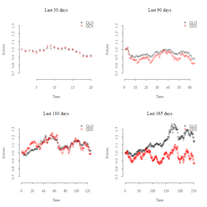
You can see the two ETF’s follow closely. This plots is basically what you get from google finance, they were scaled to show returns with respect to some date. Now, the plan is to long one and short the other when they drift too far apart. What’s the problem then?

The bottom right plot shows the GLD has been performing much better than GDX over the last year, (252 trading days). I want to short GLD and to long GDX and to sit on it until convergence. How much should I long and how much should I short? one to one? surely wrong as the price of GDX is 52.68 and the price of GLD is 155.23. Maybe equate the amount of stocks so that I am long and short  exactly 10000 dollar in each ETF, so long 188 GDX and short 64 GLD. However, is it the case that 1% increase in one is followed by 1% in the other? Thing is, if GLD rises 1% and GDX rises 1.5% as a result, then I need to hold 1.5 times GLD to keep my spread constant, this is important. As an example, say I hold same value, short GLD 10000 and long GDX 10000, but the relation between these two is such that when GDX rises 1% GLD rises 1.5%. What happens to my P&L when they co-move upwards? I am at a loss of 0.5%, since I am short GLD which went up more than GDX…

What people are doing to solve this is to estimate the relation between the two components. They do that using the regression: is then the amount I need from to compensate on the move of . Great, we should be up and running soon. 

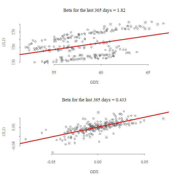
This approach, despite its appeal is far from “tried and true”. Firstly, should we use returns or actual prices? Academy likes the former, practitioners, the latter. It’s not the same in case you were wondering:

The upper plot is the estimation based on prices, it shows I should long 1.82 GLD for every 1 GDX.The bottom plot shows the same estimation based on returns, here I should hold twice GDX since every percent in GDX followed on average by only 0.433% in GLD.

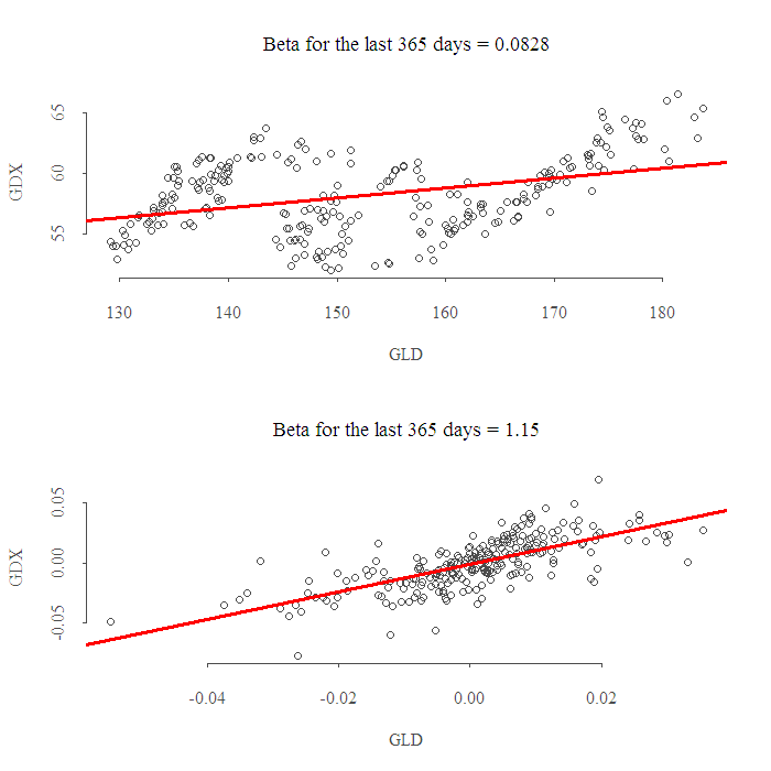
What’s more, the aforementioned regression is infected with the underlying assumption that the right hand side variable is constant while the left hand side variable is random, it has an error term. In fact, is also random, so when we switch the variables in the regression, plugging GDX on the “Y” side we get different results:

This is disturbing, the amount I should trade is determined by the order in which I plug in the variables?? Does not sound like a money machine to me. Remember, I do not care that GLD is the one dragging GDX, (gold is dragging gold miners and not the reverse), all I am saying is that GLD is not a given constant, but a random variable in its own right.

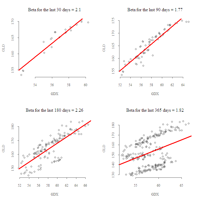
To make matters more interesting, is not constant over time, so I have no idea how many observation to use.Have a look:

This is of course the case for returns as well, and if you reverse the order of the LHS and RHS variables. You can copy paste the code and try it yourself, it’s pretty much a stand alone code.

Possible solutions are to think about your time horizon for investment, so for example if you plan to hold if for few months you can use the 365 days beta. I also tried to weight the observations such that the most recent get more weight and such other variations, did not reach any satisfactory condition to determine as to how much I should hold from each.

In theory, there is a strong relation between theory and practice, but in practice there is not. I showed here few the problems in pairs trading. Firstly, we do not know which measure to use for relation estimation, prices or returns. Secondly, we do not know which time frame to use and since the relation is not constant, it does matter.Lastly, the assumptions underlying the estimation procedure are false and invalidate whatever you hoped to feel comfortable with. As always, code and references are given below. Thanks for reading.

[asa mytpl]0470284889[/asa]

[asa mytpl]0375758259[/asa]

[asa mytpl]0470848855[/asa]

[asa mytpl]0471460672[/asa]

R code: