Omitted Variable Bias

Frequently, we see the term ‘control variables’. The researcher introduces dozens of explanatory variables she has no interest in. This is done in order to avoid the so-called ‘Omitted Variable Bias’.

What is Omitted Variable Bias?

In general, OLS estimator has great properties, not the least important is the fact that for a finite number of observations you can faithfully retrieve the marginal effect of X on Y, that is $E(\widehat{\beta}) = \beta$ . This is very much not the case when you have a variable that should be included in the model but is left out. As in my previous posts about Multicollinearity and heteroskedasticity, I only try to provide the intuition since you are probably familiar with the result itself.

For illustration, consider the model

$\begin{align*} y_t = x_{1,t}+x_{2,t} + \varepsilon_t, \end{align*}$

So Y is the sum, i.e. $\beta_1 = \beta_2 = 1$ . What happens to our estimate for $\beta_1$ when we do not include $x_2$ in the model? Mathematically we get the simple result*:

$\begin{align*} E(\widehat{\beta}_1) = \beta_1 + \beta_2 \times \widehat{\gamma}_1. \end{align*}$

The second term on the RHS is bad news. $\widehat{\gamma}_1$ is the estimate of the coefficient from the (hypothetical) equation

$\begin{align*} x_{2,t} = \gamma_0 + \gamma_1 x_{1,t} + \nu_t. \end{align*}$

In words, the term $\beta_2 \times \widehat{\gamma}_1$ represents the bias. It is influenced by:
1.
The real unknown value of $\beta_2$ . If the real effect of $x_2$ on Y is absolute small, it pushes the combined term to zero and bias is small.
2.
How closely related are $x_2$ to $x_1$ . This is less trivial, if the $x_2$ has nothing to do with $x_1$ and you are lucky to get the estimate $\widehat{\gamma}_1$ to show it, the multiplicand goes to zero and bias is small. You need to be lucky since the estimate (and hence the bias) depends on the actual sample you have, you can be unlucky and get an absolute large estimate even when the X’s are independent in the population level. This subtlety can be better stated in classical textbooks.

Now, why is this so? The unaccounted-for influence of $x_2$ on Y, pushes through anyway. Mr. $x_2$ tells himself that if he is out, he is going to do what he can from the outside. He talks to $x_1$ and depending on (as in the dry formulas), how muscular is Mr. $x_2$ (real value of $\beta_2$ ) and the nature of their relationship (as in 2 above), $x_1$ is going to accommodate $x_2$ with his request. If they do not know each other, i.e. correlation is zero, $x_1$ will ignore this harassment and the bias is unlikely to be strong.

Illustration of Omitted Variable Bias

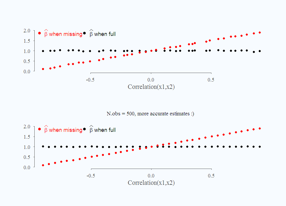
For a couple of more important insights, I need to make an illustration:


# Help function one:
hfun1 <- function(TT = 50, niter = 100, cc){
cof_full <- cof_missing <- matrix(nrow = niter, ncol = 2)
corr <- NULL
for (i in 1:niter){
# simulate from multivariate normal:
Sim.sig <- matrix(c(1,cc,cc,1),2,2 )
Sim.x  <- mvrnorm(n = TT, mu=rep(1,2), Sigma=Sim.sig)
	x1 <- Sim.x[,1]
	x2 <- Sim.x[,2]
corr[i] <- cor(x1,x2)
y <- x1 + x2 + rnorm(TT)
lm_full <- lm(y~x1+x2)
lm_missing <- lm(y~x1)
cof_full[i,] <- summary(lm_full)$coef[2,1:2] # Extract estimate and SD of estimate
cof_missing[i,] <- summary(lm_missing)$coef[2,1:2]
}
list(cof_full = cof_full, cof_missing = cof_missing, correl = corr)
}
# Run this function, once with 50 observations, once with 500.
seqq1 <- seq(-.9,.9,.05)
L <- list()
Lcorrel <-Lestimate1  <- Lstd1 <-Lestimate2  <- Lstd2 <- NULL
stdestimate1 <- stdestimate2 <- stdstdestimate1 <- stdstdestimate2 <- NULL
for (i in 1:length(seqq1))
	{
L[[i]] <- hfun1(TT = 500,  cc = seqq1[i]) 	
Lcorrel[i] <- mean(L[[i]]$correl)
Lestimate1[i] <- mean(L[[i]]$cof_full[,1])
Lstd1[i] <-  sd(L[[i]]$cof_full[,1]) 
Lestimate2[i] <- mean(L[[i]]$cof_missing[,1])
Lstd2[i] <- sd(L[[i]]$cof_missing[,1])  
stdestimate1[i] <- mean(L[[i]]$cof_full[,2])  
stdestimate2[i] <- mean(L[[i]]$cof_missing[,2])  
stdstdestimate1[i] <- sd(L[[i]]$cof_full[,2]) 
stdstdestimate2[i] <- sd(L[[i]]$cof_missing[,2]) 
}

# Help function one:

hfun1 <- function(TT = 50, niter = 100, cc){

cof_full <- cof_missing <- matrix(nrow = niter, ncol = 2)

corr <- NULL

for (i in 1:niter){

# simulate from multivariate normal:

Sim.sig <- matrix(c(1,cc,cc,1),2,2 )

Sim.x <- mvrnorm(n = TT, mu=rep(1,2), Sigma=Sim.sig)

x1 <- Sim.x[,1]

x2 <- Sim.x[,2]

corr[i] <- cor(x1,x2)

y <- x1 + x2 + rnorm(TT)

lm_full <- lm(y~x1+x2)

lm_missing <- lm(y~x1)

cof_full[i,] <- summary(lm_full)$coef[2,1:2] # Extract estimate and SD of estimate

cof_missing[i,] <- summary(lm_missing)$coef[2,1:2]

}

list(cof_full = cof_full, cof_missing = cof_missing, correl = corr)

}

# Run this function, once with 50 observations, once with 500.

seqq1 <- seq(-.9,.9,.05)

L <- list()

Lcorrel <-Lestimate1 <- Lstd1 <-Lestimate2 <- Lstd2 <- NULL

stdestimate1 <- stdestimate2 <- stdstdestimate1 <- stdstdestimate2 <- NULL

for (i in 1:length(seqq1))

{

L[[i]] <- hfun1(TT = 500, cc = seqq1[i])

Lcorrel[i] <- mean(L[[i]]$correl)

Lestimate1[i] <- mean(L[[i]]$cof_full[,1])

Lstd1[i] <- sd(L[[i]]$cof_full[,1])

Lestimate2[i] <- mean(L[[i]]$cof_missing[,1])

Lstd2[i] <- sd(L[[i]]$cof_missing[,1])

stdestimate1[i] <- mean(L[[i]]$cof_full[,2])

stdestimate2[i] <- mean(L[[i]]$cof_missing[,2])

stdstdestimate1[i] <- sd(L[[i]]$cof_full[,2])

stdstdestimate2[i] <- sd(L[[i]]$cof_missing[,2])

}

Omitted Variable Bias — The fact that you have more 500 instead of 50 observation does absolutely nothing to mitigate this problem. This is to say that the estimate is not only biased but also inconsistent, which means we can not get around this problem it easily.

Finally, have a look at this absurd situation, I plot the standard deviation of the estimate when there is a bias and when there isn’t:

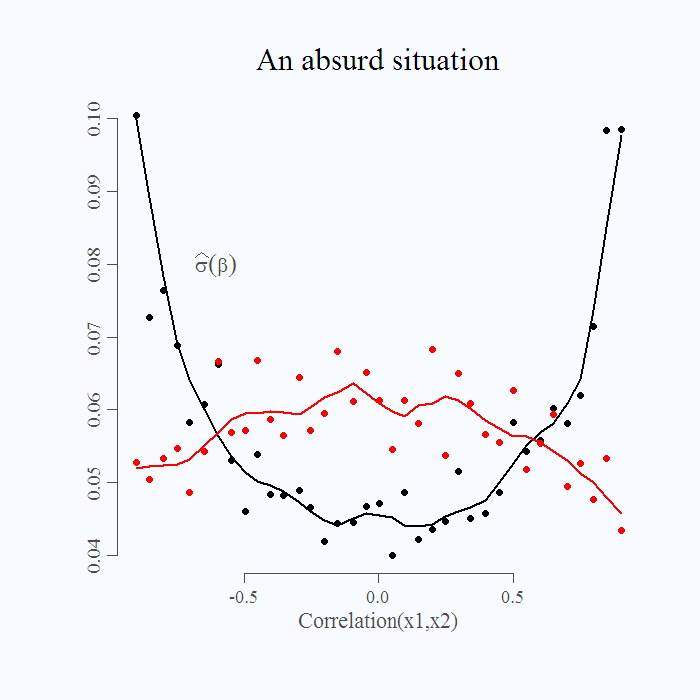
Standard Deviation when OV — In black, the standard deviation when the model is correctly specified. The parabolic shape is due to multicollinearity. In red is the (estimated) standard deviation of the incorrectly specified model.

It is absurd. When the bias is small, around zero, we find it harder to estimate the parameter (standard deviation of the estimate is relatively high). On the other hand, when the bias is strong, standard deviation is lower. When the the model is more severely misspecified, we get a more accurate estimate. Talk about the dangerous inference.

* Derivation in page 149 of this book.

You might also like:

What is Omitted Variable Bias?

Illustration of Omitted Variable Bias

You might also like:

Leave a Reply