Roughly speaking, Multicollinearity occurs when two or more regressors are highly correlated. As with heteroskedasticity, students often know what does it mean, how to detect it and are taught how to cope with it, but not why is it so. From Wikipedia: “In this situation (Multicollinearity) the coefficient estimates may change erratically in response to small changes in the model or the data.” The Wikipedia entry continues to discuss detection, implications and remedies. Here I try to provide the intuition.
You can think about it as an identification issue. If , and you estimate
how can you tell is is moving due to
or due to
? If you have a perfect Multicollinearity, meaning
your software will just refuse to even try.
For illustration, consider the model
so it is hard to get the correct ‘s, in this case,
.
The following function generate data from this model, using a “cc” parameter which determines how correlated are the two x’s.
|
1 2 3 4 5 6 7 8 9 10 11 12 13 14 15 16 |
hfun1 <- function(TT = 50, niter = 100, cc){ cof1 <- cof2 <- matrix(nrow = niter, ncol = 2) corr <- NULL for (i in 1:niter){ x1 <- rnorm(TT,5,1) x2 <- x1 + rnorm(TT,0,cc) corr[i] <- cor(x1,x2) y <- x1 + x2 + rnorm(TT) lm0 <- lm(y~x1+x2) cof1[i,] <- summary(lm0)$coef[2,1:2] # Extract estimate and SD of estimate cof2[i,] <- summary(lm0)$coef[3,1:2] } list(x1.coef = cof1, x2.coef = cof2, correl = corr) } |
Now we generate many, using a sequence which controls the correlation:
|
1 2 3 4 5 6 7 8 9 10 11 12 13 14 15 16 17 18 19 20 21 |
seqq1 <- seq(.9,0.2,-.01) L <- list() Lcorrel <-Lestimate1 <- Lstd1 <-Lestimate2 <- Lstd2 <- NULL stdestimate1 <- stdestimate2 <- stdstdestimate1 <- stdstdestimate2 <- NULL for (i in 1:length(seqq1)){ L[[i]] <- hfun1(cc = seqq1[i]) Lcorrel[i] <- mean(L[[i]]$correl) Lestimate1[i] <- mean(L[[i]]$x1.coef[,1]) Lstd1[i] <- sd(L[[i]]$x1.coef[,1]) Lestimate2[i] <- mean(L[[i]]$x2.coef[,1]) Lstd2[i] <- sd(L[[i]]$x2.coef[,1]) stdestimate1[i] <- mean(L[[i]]$x1.coef[,2]) stdestimate2[i] <- mean(L[[i]]$x2.coef[,2]) stdstdestimate1[i] <- sd(L[[i]]$x1.coef[,2]) stdstdestimate2[i] <- sd(L[[i]]$x2.coef[,2]) } |
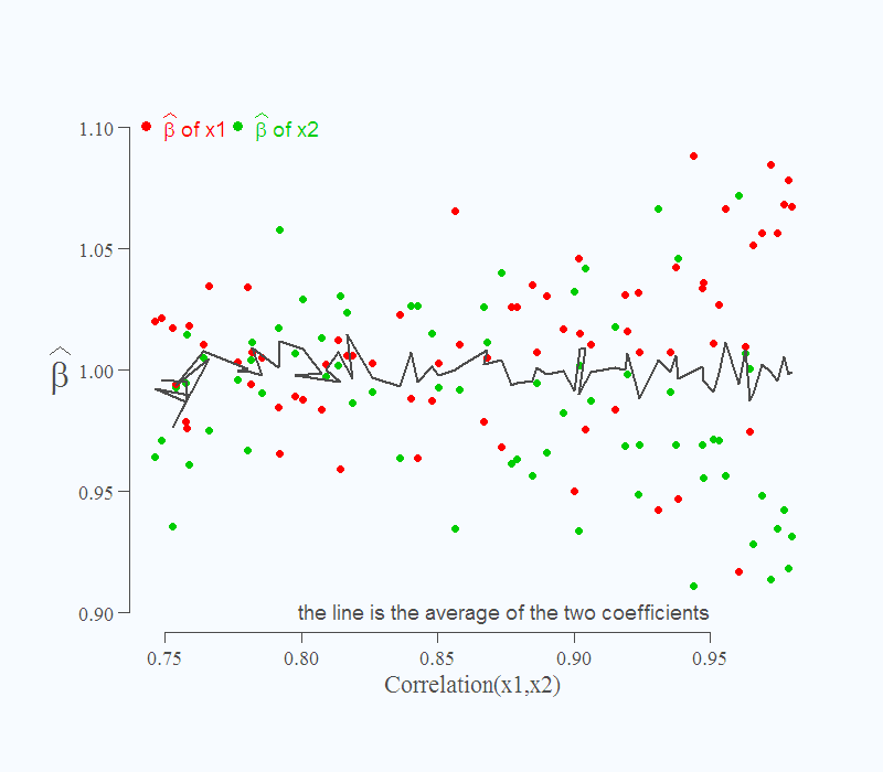
To produce the following figure:

It is also known that if you do not care to make inference, but only interested in point forecast, you need not concern yourself. This is shown via the solid line. Despite the difficulty in estimating the individual effects, the over all, or in this case, their sum is correct, still 2 as it should be.
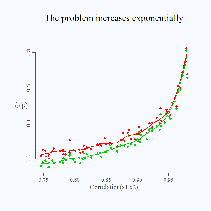
How severe is the problem depends of course on the degree of collinearity, higher degree, the more problematic the situation. It is not a linear increase:
 You can see that even if correlation is around 0.8, inference is limited but perhaps manageable. As we move up in correlation, the standard deviation of the estimate is getting ridiculously high, in a sense that the estimate is 1, but it can be quite easily estimated as 0 or 2. This is shown by the increased standard deviation of the estimate, especially the sharp increase when correlation is above 0.95.
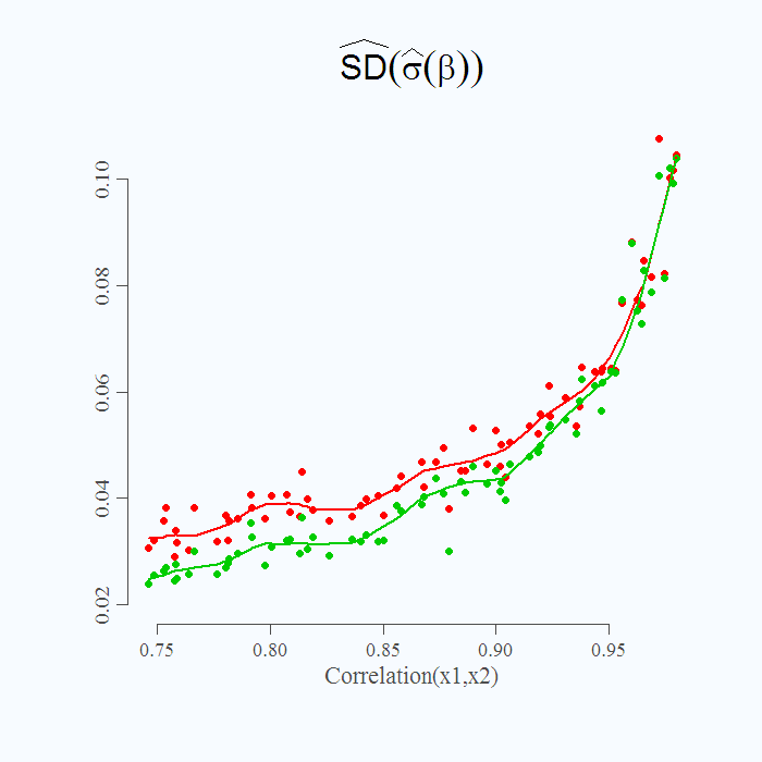
Finally and a bit more delicate, what is plotted in figure 2 is not the actual standard deviation but an estimate of the real unobserved standard deviation parameter. Since we already simulated 50 iterations per setting, we can have a look at the simulation variance of this estimate. In the code above it is specified as “stdstdestimate” which is the standard deviation of the many standard deviation we get for each correlation value specified.  Note the Y axis, what is plotted now is the (simulation) standard deviation of the estimate for the standard deviation of the
 ‘s. It is a higher order examination (variance of variance). What it shows is that you know that you know less (higher standard deviation for
) but also that you are less sure, how much less you know (higher standard deviation of your estimate for the standard deviation of
). Fattening food for thought.


collinearity is a big topic discussed in my book
Hands-On Intermediate Econometrics Using R: Templates for Extending Dozens of Practical Examples
Its index has several references to ridge regression as a tool for handling collinearity
eigenvalues of X’X close to but not equal to 0 leads to near collinearity. This is arguably more harmful than perfect collinearity since the latter will be caught beforehand.
best wishes
Hi Hrishikesh,
Your book is on my shelf, its high ranking is justified.
Nicely done!
Very useful!
Can you explain, please, what do you mean in Figure 1 by saying “…the tougher it is to distinguish which is which”? Do you mean which green and red dot are in pair?
Sure: because of the higher correlation between the variables, it is hard for the regression to disentangle whether Y moves due to the change in x1, or due to the change in x2. As you move to the right in the figure you mentioned, the explanatory variables co-move more closely, so it is hard to distinguish between them. For example, it happens more often that the machine decides to assign a value of 1.1 to beta_1 (the impact of the x1) and 0.9 to beta_2 (the impact of x2); by that, implicitly giving x1 more influence over the fitted value. This happens because the machine concludes some of the effect which actually comes from x2, is attributed to x1 (again, because it is hard to distinguish between them in that region).