Correlation and correlation structure (7) – Chatterjee's rank correlation

Remarkably, considering that correlation modelling dates back to 1890, statisticians still make meaningful progress in this area. A recent step forward is given in A New Coefficient of Correlation by Sourav Chatterjee. I wrote about it shortly after it came out, and it has since garnered additional attention and follow-up results. The more I read about it, the more I am impressed with it. This post provides some additional details based on recent research.

What is Chatterjee’s rank correlation?

The formula for Chatterjee’s rank correlation:

$\xi_{n}(X, Y):=1-\frac{3 \sum_{i=1}^{n-1}\left|r_{i+1}-r_{i}\right|}{n^{2}-1}$

$r_i$ is the rank of $Y_i$ and $X$ is rearranged to be order $X_{(1)} \leq \cdots \leq X_{(n)}$ .

Briefly: do, on average, larger values of $X_i$ drag a higher ranking for $Y_i$ ? yeah –> high correlation, no? –> low correlation.

Reasons to like:

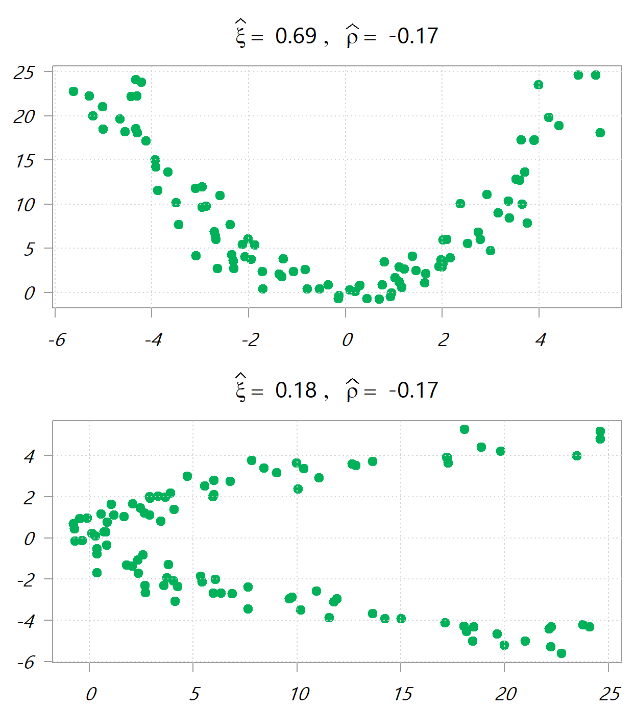
Asymmetry. It’s possible that $y = f(x)$ , but $x \neq f(y)$ and it’s nice that it’s reflected.

If $x$ is random draws in [-5,5], the following images depict $y = x^2$ , once y~x and once x~y. Values in the headers are the new ranking-based correlation measure and the traditional Pearson correlation measure.

Symmetry? Why not?

Say you want just a measure for the dependency between two variables, and you don’t care what drives the dependency. No problem. Just as the Jensen-Shannon divergence symmetric divergence is simply the average of two Kullback-Leibler asymmetric divergences, so here you can just use $\xi = \frac{\xi(Y,X) + \xi(X,Y) }{2}.$

Reasons to dislike:

Inference only through asymptotic analysis

From a recent Biometrika paper:

… the standard bootstrap, in general, does not work for Chatterjee’s rank correlation. … Chatterjee’s rank correlation thus falls into a category of statistics that are asymptotically normal but bootstrap inconsistent.

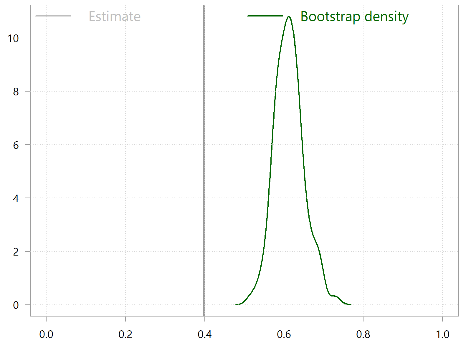
This means that you shouldn’t use bootstrap for any inference or significance testing. The following simple code snippets reveals the problem:


# install.packages("XICOR")
# citation("XICOR")
library(XICOR)

tt <- 100
x <- runif(tt,-5,5)
sdd <- 1
x2 <- x^2 + rnorm(tt, sd=sdd)
x1 <- x + rnorm(tt, sd=sdd)
samplexi <- calculateXI(x1,x2) 
samplexi
bootxi <- NULL
for (i in 1:tt) {
  tmpind <- sample(tt, replace = T)
    bootxi[i] <- calculateXI(x1[tmpind],x2[tmpind])
}
density(bootxi) %>% 
plot(xlab="", main="", xlim = c(0,1), ylab="", lwd=2, col="darkgreen")
abline(v= samplexi, lwd=3)
grid()

# install.packages("XICOR")

# citation("XICOR")

library(XICOR)

tt <- 100

x <- runif(tt,-5,5)

sdd <- 1

x2 <- x^2 + rnorm(tt, sd=sdd)

x1 <- x + rnorm(tt, sd=sdd)

samplexi <- calculateXI(x1,x2)

samplexi

bootxi <- NULL

for (i in 1:tt) {

tmpind <- sample(tt, replace = T)

bootxi[i] <- calculateXI(x1[tmpind],x2[tmpind])

}

density(bootxi) %>%

plot(xlab="", main="", xlim = c(0,1), ylab="", lwd=2, col="darkgreen")

abline(v= samplexi, lwd=3)

grid()

Bootstrap fails miserably here. What you see is that the density of the bootstrapped statistic is completely off the mark in that it’s not even centered around the sample-estimate. So, you can’t use bootstrap for inference, and you must also avoid any other procedures that are bootstrap-driven (e.g. bagging). This is the end of the post if you don’t care why bootstrap fails here.

Why bootstrap fails in this case?

10 years ago I gave this example for a bootstrap failure. Back then I did not know the reason for this, but now I know enough. It has to do with statistics which are not smooth with respect to the data.

A statistic $T$ of a dataset $X=\left\{x_1, x_2, \ldots, x_n\right\}$ is considered $k$ -smooth if it has $k$ continuous derivatives with respect to each data point $x_i$ . Formally, this means that for any data point $x_i$ in $X$ , the partial derivatives $\frac{\partial T}{\partial x_i}, \frac{\partial^2 T}{\partial x_i^2}, \ldots, \frac{\partial^k T}{\partial x_i^k}$ exist, and are continuous for all $k \geq 1$ . Bootstrap only works for smooth statistics, which qualifies for most of what you are familiar with, e.g. mean and variance. Bu ranking changes in a stepwise fashion rather than smoothly. So when we bootstrap, rankings “jump” rather than “crawl” which troubles the bootstrapping technique. The example I gave a decade ago spoke of the maximum. The derivative is not continuous in that or it’s 0 (no change in the maximum), or it jumps to a different value, so that is why we can’t use bootstrap (at least not the standard nonparametric version).

References

Bootstrap Methods and Their Application

Reshef,D.N., Reshef, Y. A., Finucane, H. K.,Grossman, S. R.,McVean, G., Turnbaugh, P. J., Lander, E. S., Mitzenmacher, M., and Sabeti, P. (2011), “Detecting Novel Associations in Large Datasets” Science, 334, 1518–1524.

R package XICOR: Association Measurement Through Cross Rank Increments
Applied Multiple Regression/Correlation Analysis for the Behavioral Sciences

You might also like:

One comment on “Correlation and correlation structure (7) – Chatterjee’s rank correlation”

Staffan Betnér says:

03/22/2024 at 8:57 PM

The “Bayesian” (aka fractional (random) weighted bootstrap) bootstrap works, though. At least it works in the sense that larger samples give narrower bootstrap distributions, and the mean of the bootstrap distribution is very close to the point estimate.

What is Chatterjee’s rank correlation?

Why bootstrap fails in this case?

References

You might also like:

One comment on “Correlation and correlation structure (7) – Chatterjee’s rank correlation”

Leave a Reply