Many years ago, when I was still trying to beat the market, I used to pair-trade. In principle it is quite straightforward to estimate the correlation between two stocks. The estimator for beta is very important since it determines how much you should long the one and how much you should short the other, in order to remain market-neutral. In practice it is indeed very easy to estimate, but I remember I never felt genuinely comfortable with the results. Not only because of instability over time, but also because the Ordinary Least Squares (OLS from here on) estimator is theoretically justified based on few text-book assumptions, most of which are improper in practice. In addition, the OLS estimator it is very sensitive to outliers. There are other good alternatives. I have described couple of alternatives here and here. Here below is another alternative, provoked by a recent paper titled Adaptive Huber Regression.
Huber Regression
The paper Adaptive Huber Regression can be thought of as a sequel to the well established Huber regression from 1964 whereby we adapt the estimator to account for the sample size.
OLS penalizes all residuals with their squared, and it is this which creates the sensitivity of this estimator; large deviations have exponentially increasing impact. If we give the OLS a chill pill, it would not react so strongly to very large deviations. Here is an image for different “reaction” function:
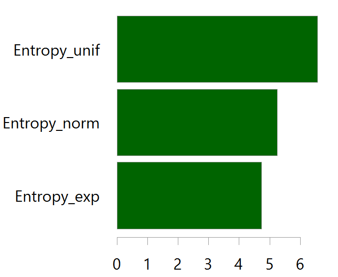
You can see for example the Least Absolute Deviation (LAD) penelizes a deviation of 3 with a loss of 3, while the OLS penelizes a deviation of 3 with a loss of 9. The OLS minimizes the sum of squared residuals. The LAD minimizes the sum of absolute residuals. The Huber loss function depends on a hyper parameter which gives a bit of flexibility.
The Huber loss function can be written as*:

In words, if the residuals in absolute value ( here) are lower than some constant (
 here) we use the “usual” squared loss. But if the residuals in absolute value are larger than , than the penalty is larger than , but not squared (as in OLS loss) nor linear (as in the LAD loss) but something we can decide upon. The parameter controls the blending between the usual quadratic loss for small deviations and a less rigid loss for larger deviations. It is sometimes referred to as a robustification parameter. The thrust of the paper Adaptive Huber Regression (link to paper) is that the author condition the value on the sample size, which is a nice idea.
Couple of more attention points. Point one: while OLS assigns equal weight to each observation, the Huber loss assigns different weights to each observation. So the estimate for  can be written as**

which regrettably means that the estimate depends on itself in a way, because the residuals depends on the estimate. This prevents us from obtaining a closed-form solution, and so we need to use a numerical method called iteratively reweighted least-squares. Point two: because we specify a particular loss function, and for a particular choices of the tuning parameter we can be left with familiar canonical distribution, the estimation can be considered as a generalization of maximum-likelihood estimation method, hence it is referred to as “M”-estimation.
Huber Regression in R
In this section we will compare the Huber regression estimate to that of the OLS and the LAD. Assume you want to take a position in a company (ticker BAC below), but would like to net out the market impact. So it would be like pair-trade the particular name and the market (ticker SPY below):
# packages needed
library(quantmod)
library(magrittr)
library(quantreg)
library(MASS)
end= format(Sys.Date(),"%Y-%m-%d")
start= format(as.Date("1998-09-18"),"%Y-%m-%d")
dat0 = getSymbols("BAC", src="yahoo", from=start, to=end, auto.assign = FALSE) %>% as.matrix
dat1 = getSymbols("SPY", src="yahoo", from=start, to=end, auto.assign = FALSE) %>% as.matrix
NROW(dat0)== NROW(dat1) # check if both tickers contain all days
n <- NROW(dat0)
ret = (dat0[2:n, 4]/dat0[1:(n-1),4] - 1) # BAC returns
ret_spy = (dat1[2:n, 4]/dat1[1:(n-1),4] - 1) # SPY retuns
bet = lm(ret~ret_spy)$coef[2] # OLS beta
rbet = rq(ret~ret_spy)$coef[2] # Robust beta
huber_reg = rlm(y= ret, x= ret_spy, method= "M", scale.est= "Huber")
summary(huber_reg)
hbet <- huber_reg$coef # Huber beta
Results
| Beta | |
|---|---|
| OLS | 1.53 |
| LAD | 1.21 |
| Huber | 1.28 |
As you can see the Huber estimate sits in this case between the estimate of the LAD and the OLS estimate. What happens is that the computer solves those equations above and re-weight the observation.
plot(ret, huber_reg$w)
An illustration:
The resulting weights (y) over the returns of the BAC (x)
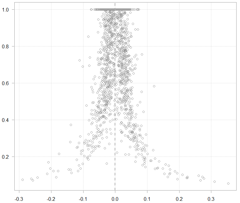
The chart above is just for illustration, the weights are calculated not based on  alone but based on
  , but I thought it is good to show to get the intuition behind what the machine actually does.
This is how it looks when we plot the three regression lines on a scatter plot:
Scatter plot of BAC returns over the SPY returns, with overlaid different regression lines
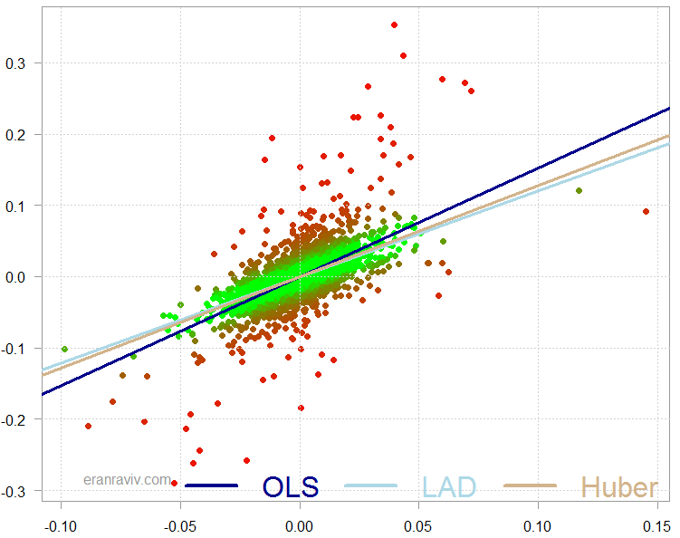
The chart is colored such that the more red the point, the lower the weight it was given in the overall estimation.
The Huber regression is good balance between simply removing the outliers, and ignoring them. You can tune the amount of influence you would like to have in the overall estimation, by that giving room for those observations without allowing them “full pull” privileges.
References
Adaptive Huber Regression (link to paper)
Outliers and Loss Functions
Footnotes
* Sometimes the loss function is being divided by 2, but for it’s irrelevant, it doesn’t change the optimization solution.
** We usually scale the residuals


For pairs trading, correlation is the wrong tool. Cointegration is what should be used instead.
Thanks for the comment Mike. Good point. If done on returns as it is in this post, the vector (1, beta) is also the cointegration vector; and the beta in this univariate regression is the same as the (Pearson) correlation, so me writing correlation is like you writing cointegration, in this special case.