The covariance matrix is central to many statistical methods. It tells us how variables move together, and its diagonal entries – variances – are very much our go-to measure of uncertainty. But the real action lives in its inverse. We call the inverse covariance matrix either the precision matrix or the concentration matrix. Where did these terms come from? I’ll now explain the origin of these terms and why the inverse of the covariance is named that way. I doubt this has kept you up at night, but I still think you’ll find it interesting.
Why the Inverse Covariance is Called Precision?
Variance is just a noisy soloist, if you want to know who really controls the music – who depends on whom – you listen to precision  . While a variable may look wiggly and wild on its own, you often can tell where it lands precisely, conditional on the other variables in the system. The inverse of the covariance matrix encodes the conditional dependence any two variables after controlling the rest. The mathematical details appear in an earlier post and the curious reader should consult that one.
Here the following code and figure provide only the illustration for the precision terminology. Consider this little experiment:
![\[ X_2, X_3 \sim \mathcal{N}(0,1) \text{, independent and ordinary.} \]](https://eranraviv.com/wp-content/ql-cache/quicklatex.com-77932a40aed9b8a19f8cbed462a126fc_l3.svg "Rendered by QuickLaTeX.com")
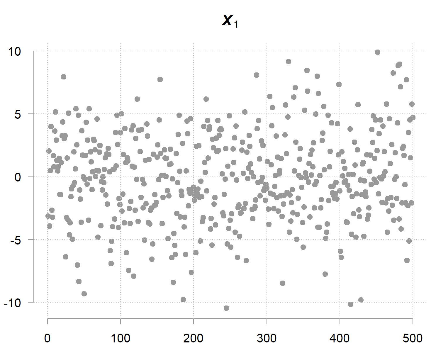
![\[ X_1 = 2X_2 + 3X_3 + \text{small noise}.\]](https://eranraviv.com/wp-content/ql-cache/quicklatex.com-f977845f0df331204b7bb8e60c7d1d32_l3.svg "Rendered by QuickLaTeX.com")
Now,  has a large variance (marginal variance), look, it’s all over the place:
But but but… given the other two variables you can determine quite accurately (because it doesn’t carry much noise on its own); hence the term precision. The precision matrix captures exactly this phenomenon. Its diagonal entries are not about marginal uncertainty, but conditional uncertainty; how much variability remains when the values of the other variables are given. The inverse of the precision entry  is the residual variance of after regression it on the other two variables. The math behind it is found in an earlier post, for now it’s suffice to write:
![\[\text{For each } i=1,\dots,n: \quad X_i = \sum_{j \neq i} \beta_{ij} X_j + \varepsilon_i, \quad \text{with } \mathrm{Var}(\varepsilon_i) = \sigma_i^2.\]](https://eranraviv.com/wp-content/ql-cache/quicklatex.com-b2117260325064797f25890f8fab0508_l3.svg "Rendered by QuickLaTeX.com")
![\[\quad \Omega_{ii} = \tfrac{1}{\sigma_i^2}, \qquad \Omega_{ij} = -\tfrac{\beta_{ij}}{\sigma_i^2}.\]](https://eranraviv.com/wp-content/ql-cache/quicklatex.com-dff21eed569b6f91345eab16be17be60_l3.svg "Rendered by QuickLaTeX.com")
So after accounting for the other two variables, you are left with
![\[\text{small noise} --> \frac{1}{\text{small noise}} --> \text{high precision}\]](https://eranraviv.com/wp-content/ql-cache/quicklatex.com-706b578fc06d4f88ca98130a113929b6_l3.svg "Rendered by QuickLaTeX.com")
which in this case looks as follows:
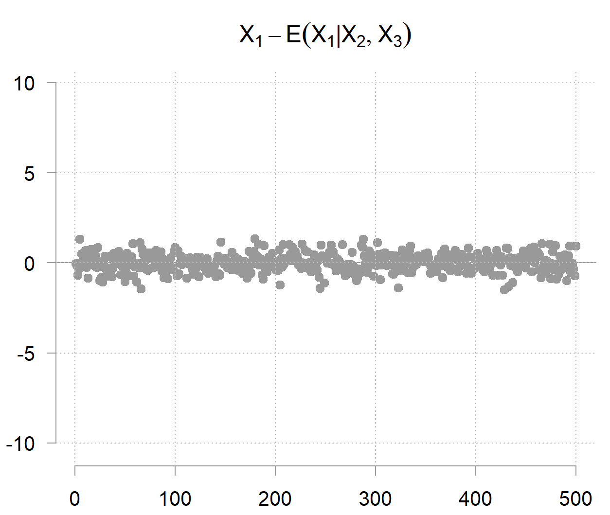
This small illustration also reveals a useful computational insight. Instead of directly inverting the covariance matrix (expensive for high dimensions), you can also run parallel regressions of each variable on all others, which may scale better on distributed systems.
Why the Inverse Covariance is Called Concentration?
Now, what motivates the concentration terminology? What is concentrated? Let’s unwrap it. Let’s begin by first looking at the density of a single normally distributed random variable:
![\[f(x) \propto \exp\left(-\frac{1}{2}\frac{(x-\mu)^2}{\sigma^2}\right).\]](https://eranraviv.com/wp-content/ql-cache/quicklatex.com-d12845f6dc510c93daf6e0b6b43110e1_l3.svg "Rendered by QuickLaTeX.com")
So if  we have
  , and otherwise we have
  . This negative number will then be divided by the variance, or, in our context multiplied by the precision (which is the reciprocal of the variance for a single variable). A higher precision value makes for a negativier (😀) exponent. In turn, it reduces the overall density the further we drift from the mean (think faster mass-drop in the tails), so a sharper, more peaked density where the variable’s values are tightly concentrated around the mean. A numeric sanity check. Below are two cases with mean zero, one with variance 1 (so precision
  ), and the other with variance 4 (
 ). We look at two values, one at the mean (
 ), and one farther away (
 ), and check the density mass at those values for the two cases (
 ,
,  , and
, and  and
and  ) :
) :
![\[ X\sim\mathcal N(0,\sigma^2),\quad \tau=\frac{1}{\sigma^2},\quad p_\tau(x)=\frac{\sqrt{\tau}}{\sqrt{2\pi}}\exp\!\left(-\tfrac12\tau x^{2}\right) \]](https://eranraviv.com/wp-content/ql-cache/quicklatex.com-aabaea98c484ccef3dea700526e07de1_l3.svg "Rendered by QuickLaTeX.com")
![\[ p_{1}(0)=\frac{1}{\sqrt{2\pi}}\approx 0.39,\qquad p_{4}(0)=\frac{2}{\sqrt{2\pi}}=\sqrt{\frac{2}{\pi}}\approx 0.79 \]](https://eranraviv.com/wp-content/ql-cache/quicklatex.com-5d4963796d413f0ebb6d04f1fd592853_l3.svg "Rendered by QuickLaTeX.com")
![\[ p_{1}(1)=\frac{1}{\sqrt{2\pi}}e^{-1/2}\approx 0.24,\qquad p_{4}(1)=\frac{2}{\sqrt{2\pi}}e^{-2}\approx 0.10 \]](https://eranraviv.com/wp-content/ql-cache/quicklatex.com-2d268a7c77b892aeb7da70f4589570b2_l3.svg "Rendered by QuickLaTeX.com")
![\[ \tau\uparrow\;\Rightarrow\;p(0)\uparrow,\;p(1)\downarrow \]](https://eranraviv.com/wp-content/ql-cache/quicklatex.com-ff5b9448befd6ebf47c4e8839bcdd878_l3.svg "Rendered by QuickLaTeX.com")
In words: higher precision leads to lower density mass away from the mean and, therefore, higher density mass around the mean (because the density has to sum up to one, and the mass must go somewhere).
Moving to the multivariate case. Say that also is normally distributed, then the joint multivariate Gaussian distribution of our 3 variables is proportional to:
![\[f(\mathbf{x}) \propto \exp\!\left(-\tfrac{1}{2}(\mathbf{x}-\boldsymbol{\mu})^\top \mathbf{\Omega} (\mathbf{x}-\boldsymbol{\mu})\right)\]](https://eranraviv.com/wp-content/ql-cache/quicklatex.com-075f7d1e6f5c0d652bf2dd293cdcb212_l3.svg "Rendered by QuickLaTeX.com")
![\[\mathbf{x} = \begin{bmatrix} x_1 \\ x_2 \\ x_3 \end{bmatrix}, \quad \boldsymbol{\mu} = \begin{bmatrix} \mu_1 \\ \mu_2 \\ \mu_3 \end{bmatrix}, \quad \mathbf{\Omega} = \begin{bmatrix} \Omega_{11} & \Omega_{12} & \Omega_{13} \\ \Omega_{21} & \Omega_{22} & \Omega_{23} \\ \Omega_{31} & \Omega_{32} & \Omega_{33} \end{bmatrix}\]](https://eranraviv.com/wp-content/ql-cache/quicklatex.com-804c0cbf11085fc4ddbf1932b3c6bc34_l3.svg "Rendered by QuickLaTeX.com")
In the same fashion, directly sets the shape and orientation of the contours of the multivariate density. If there is no correlation (think a diagonal ), what would you expect to see? that we have a wide, diffused, spread-out cloud (indicating little concentration). By way of contrast, a full weights the directions differently; it determines how much probability mass gets concentrated in each direction through the space.
Another way to see this is to remember that for the multivariate Gaussian density case,  appears in the nominator, so the inverse, the covariance
  would be in the denominator. Higher covariance entries means more spread, and as a result a lower density values at individual points and thus a more diffused multivariate distribution overall.
The following two simple  scenarios illustrate the concentration principle explained above. In the code below you can see that while I plot only the first 2 variables, there are actually 3 variables, but the third one is independent; so high covariance would remain high even if we account for the third variable (I say it so that you don’t get confused that we now work with the covariance, rather then with the inverse). Here are the two scenarios:

 with correlation
  creates spherical contours.

 with correlation
  creates elliptical contours stretched along the correlation direction.
Rotate the below interactive plots to get a clearer sense of what we mean by more/less concentration. Don’t forget to check the density scale.
Round hill: diffused, less concentrated
Elongated ridge: steep\peaky, more concentrated
Hopefully, this explanation makes the terminology for the inverse covariance clearer.
Code
For Precision
|
1 2 3 4 5 6 7 8 9 10 11 12 13 14 15 16 17 18 19 20 21 22 23 24 25 26 27 28 29 30 31 32 33 34 35 36 37 38 39 40 41 42 43 |
# Combine into matrix X <- cbind(X1, X2, X3) # Compute covariance and precision set.seed(123) n <- 100 # Generate correlated data where X1 has high variance but is predictable from X2, X3 # X1 = 2*X2 + 3*X3 + small noise X2 <- rnorm(n, 0, 1) X3 <- rnorm(n, 0, 1) X1 <- 2*X2 + 3*X3 + rnorm(n, 0, 0.5) # Small conditional variance! # Combine into matrix X <- cbind(X1, X2, X3) # Compute covariance and precision Sigma <- cov(X) Omega <- solve(Sigma) # Display results cat("MARGINAL variances (diagonal of Sigma):\n") print(diag(Sigma)) X1 X2 X3 11.3096683 0.8332328 0.9350631 cat("\nPRECISION values (diagonal of Omega):\n") print(diag(Omega)) X1 X2 X3 4.511182 18.066305 41.995608 cat("\nCONDITIONAL variances (1/diagonal of Omega):\n") print(1/diag(Omega)) X1 X2 X3 0.22167138 0.05535166 0.02381201 Verification - Residual variance from regression: cat("Var(X1|X2,X3) =", var(fit$residuals), "\n") Var(X1|X2,X3) = 0.2216714 cat("1/Omega[1,1] =", 1/Omega[1,1], "\n") 1/Omega[1,1] = 0.2216714 |
For Concentration
|
1 2 3 4 5 6 7 8 9 10 11 12 13 14 15 16 17 18 19 20 21 22 23 24 25 26 27 28 29 30 31 32 33 34 35 36 37 38 39 40 41 42 43 |
library(MASS) library(rgl) library(htmltools) set.seed(123) n <- 5000 mu <- c(0,0,0) # Case 1: Low correlation (round hill) Sigma1 <- matrix(c(1, 0.1, 0, 0.1, 1, 0, 0, 0, 1), 3, 3) X1 <- mvrnorm(n, mu=mu, Sigma=Sigma1) # Case 2: High correlation (elongated ridge) Sigma2 <- matrix(c(1, 0.9, 0, 0.9, 1, 0, 0, 0, 1), 3, 3) X2 <- mvrnorm(n, mu=mu, Sigma=Sigma2) # Density for marginal (X1,X2) kd1 <- kde2d(X1[,1], X1[,2], n=150, lims=c(range(X1[,1]), range(X1[,2]))) kd2 <- kde2d(X2[,1], X2[,2], n=150, lims=c(range(X2[,1]), range(X2[,2]))) # Plot 1: Low correlation → "round mountain" open3d(useNULL=TRUE) persp3d(kd1$x, kd1$y, kd1$z, col = terrain.colors(100)[cut(kd1$z, 100)], aspect = c(1,1,0.4), xlab="X1", ylab="X2", zlab="Density", smooth=TRUE, alpha=0.9) title3d("Low correlation (round, concentrated)", line=2) widget1 <- rglwidget(width=450, height=450) # Plot 2: High correlation → "ridge mountain" open3d(useNULL=TRUE) persp3d(kd2$x, kd2$y, kd2$z, col = terrain.colors(100)[cut(kd2$z, 100)], aspect = c(1,1,0.4), xlab="X1", ylab="X2", zlab="Density", smooth=TRUE, alpha=0.9) title3d("High correlation (elongated, less concentrated)", line=2) widget2 <- rglwidget(width=450, height=450) |


