Correlation and Correlation Structure (11) – Estimation using Random Matrix Theory

In the classical regime, when we have plenty of observations relative to what we need to estimate, we can rely on the sample covariance matrix as a faithful representation of the underlying covariance structure. However, in the high-dimensional settings common to modern data science – where the number of attributes/features $p$ is comparable to the number of observations $n$ , the sample covariance matrix is a bad estimator. It is not merely noisy; it is misleading. The eigenvalues of such matrices undergo a predictable yet deceptive dispersion, inflating into “signals” that have no basis in reality. But, using some machinery from Random Matrix Theory is one way to correct for biases that high-dimensional data creates.

Suppose we observe $n$ independent vectors $\mathbf{x}_1, \mathbf{x}_2, \ldots, \mathbf{x}_n$ from a $p$ -dimensional distribution with covariance matrix $\boldsymbol{\Sigma}$ . The obvious estimate is the sample covariance matrix:

$\mathbf{S} = \frac{1}{n}\sum_{i=1}^n (\mathbf{x}_i - \bar{\mathbf{x}})(\mathbf{x}_i - \bar{\mathbf{x}})^\top.$

The Problem That Won’t Go Away.

When $p$ is fixed and $n \to \infty$ , we’re in the classical regime where $\mathbf{S} \to \boldsymbol{\Sigma}$ and all is well. But modern datasets, say in genomics or finance.., routinely present us with $p \approx n$ or even $p > n$ . Here, $\mathbf{S}$ becomes a terrible estimate of $\boldsymbol{\Sigma}$ .

How terrible? Consider the eigenvalues. And remind yourself that

Each eigenvalue = variance along its eigenvector direction

Even when the true covariance is the identity matrix $\boldsymbol{\Sigma} = \mathbf{I}$ (pure noise, all eigenvalues are 1 in actuality), the eigenvalues of $\mathbf{S}$ don’t cluster near 1. Instead, they spread themselves along an interval roughly $[(1-\sqrt{p/n})^2, (1+\sqrt{p/n})^2]$ . The largest eigenvalue can be inflated by a factor of 4 when $p = n$ . This isn’t sampling variability we can ignore – it’s systematic, serious, distortion.

Enter Random Matrix Theory

Around 1967, mathematicians Marčenko and Pastur proved a remarkable theorem: as $n, p \to \infty$ with $p/n \to c \in (0,1]$ , the empirical distribution of eigenvalues of $\mathbf{S}$ converges to a specific limiting density, now called the Marčenko-Pastur law:

$f_{MP}(\lambda) = \frac{1}{2\pi c \lambda} \sqrt{(\lambda - \lambda_{-})(\lambda_{+} - \lambda)}, \quad \lambda \in [\lambda_{-}, \lambda_{+}]$

where $\lambda_{\pm} = (1 \pm \sqrt{c})^2$ – aka the bounds of the density.

This is beautiful mathematics, but what can we do with it? The key insight came from physicists (Laloux et al., 1999) studying financial correlation matrices. They noticed that most eigenvalues of real covariance matrices pile up in a “bulk” matching the Marčenko-Pastur prediction, while a few large eigenvalues stick out above. The bulk represents noise; the outliers represent signal.

A Simple Cleaning Procedure

This suggests an obvious strategy:

Identify the bulk: Estimate the noise level $\sigma^2$ and compute the Marčenko-Pastur bounds $\lambda_{\pm} = \sigma^2(1 \pm \sqrt{c})^2$

Classify eigenvalues:

Signal: $l_i > \lambda_+$ (or $l_i < \lambda_-$ if $c < 1$ )
Noise: $l_i \in [\lambda_-, \lambda_+]$

Shrink the noise: Replace noise eigenvalues with their average $\bar{l} = \frac{1}{|\text{noise}|}\sum_{i \in \text{noise}} l_i$

Reconstruct: $\tilde{\mathbf{S}} = \mathbf{U}\tilde{\mathbf{L}}\mathbf{U}^\top$ where $\tilde{\mathbf{L}}$ contains the cleaned eigenvalues

This is simple. We’re not done yet – the signal eigenvalues themselves are inflated by noise.

The Baik-Silverstein Correction

In 2006, mathematicians Baik and Silverstein analyzed the “spiked covariance model” where $\boldsymbol{\Sigma}$ has a few large eigenvalues (the “spikes”) and the rest equal to 1. They derived the precise relationship between sample and population eigenvalues. Specifically, for a signal eigenvalue $\lambda > 1 + \sqrt{c}$ , the corresponding sample eigenvalue $l$ satisfies (asymptotically):

$l \approx \lambda + \frac{c \lambda}{\lambda - 1}$
This can be inverted: given $l$ , we estimate

$\hat{\lambda} = \frac{1}{2}\left((l - c + 1) + \sqrt{(l - c + 1)^2 - 4l}\right)$

And so our $\hat{\lambda}$ can now serve as a proper estimate for the true eigenvalue in the reconstruction $\tilde{\mathbf{S}} = \mathbf{U}\tilde{\mathbf{L}}\mathbf{U}^\top$ .

Here is how it looks:

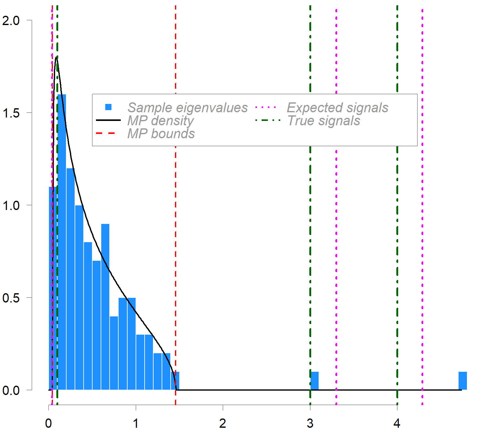
What is plotted is the empirical distribution of sample eigenvalues (blue histogram) from a 100×200 data matrix compared to the MP density (in black). The population covariance contains three (real) signal eigenvalues, indicated by the green dash-dot lines. c = 0.5 in this example. Red dashed lines mark the MP bounds. Magenta dot lines show the expected (bias-corrected) locations of sample signal eigenvalues as estimated by the inversion formula outlined above.

A valuable addition to your covariance estimation arsenal.

Code


set.seed(123)  # For reproducibility

n <- 200  # Number of observations (rows)
p <- 100  # Number of variables (columns)

# Define eigenvalues
signal_eigenvalues <- c(0.1, 3, 4)
noise_eigenvalue <- 0.5
n_signal <- length(signal_eigenvalues)

# Create the full eigenvalue vector
eigenvalues <- c(signal_eigenvalues, rep(noise_eigenvalue, p - n_signal))

# Generate random orthogonal matrix for eigenvectors
# Use QR decomposition of a random matrix
random_matrix <- matrix(rnorm(p * p), p, p)
Q <- qr.Q(qr(random_matrix))  # Orthogonal matrix (eigenvectors)

# Computes the QR decomposition of a random matrix
# Any matrix can be factored as M = QR where:
# Q is orthogonal (columns are orthonormal)
# R is upper triangular
# qr.Q Extracts just the Q matrix
# Bottom line: It's a standard trick in simulation to generate random covariance matrices with controlled eigenvalues—you specify the eigenvalues (diagonal matrix) and use a random orthogonal matrix for the directions (eigenvectors)

# Construct the population covariance matrix
Sigma <- Q %*% diag(eigenvalues) %*% t(Q)

Sigma[1:10,1:10]
# Generate data from multivariate normal with this covariance
# Mean vector is zero
mu <- rep(0, p)

# Generate the data matrix using the Cholesky decomposition
# X = Z * L where L is Cholesky factor of Sigma
L <- chol(Sigma)  # Upper triangular Cholesky factor
Z <- matrix(rnorm(n * p), n, p)  # Standard normal random variables
X <- Z %*% L  # n x p data matrix

dim(X)

# Verify the structure
cat("Data matrix dimensions:", dim(X), "\n")
cat("Population eigenvalues (first 10):", eigenvalues[1:10], "\n\n")

# Compute sample covariance matrix
S <- cov(X)

# Check sample eigenvalues
sample_eigenvalues <- eigen(S, symmetric = TRUE, only.values = TRUE)$values
cat("Sample eigenvalues (first 10):", round(sample_eigenvalues[1:10], 3), "\n")
cat("Sample eigenvalues (last 3):", round(tail(sample_eigenvalues, 3), 3), "\n\n")
barplot(sample_eigenvalues)

# Compute aspect ratio and Marchenko-Pastur bounds
c_ratio <- p / n
lambda_plus <- noise_eigenvalue * (1 + sqrt(c_ratio))^2
lambda_minus <- noise_eigenvalue * (1 - sqrt(c_ratio))^2

cat("Aspect ratio c = p/n:", round(c_ratio, 3), "\n")
cat("Marchenko-Pastur bounds for noise (sigma^2 = 0.5):", 
    round(lambda_minus, 3), "to", round(lambda_plus, 3), "\n\n")

# Expected locations of signal eigenvalues
phi <- function(lambda, c, sigma_sq = 0.5) {
  lambda_scaled <- lambda / sigma_sq
  result <- sigma_sq * (lambda_scaled + c * lambda_scaled / (lambda_scaled - 1))
  return(result)
}

# this gives us the locations of the sample eigenvalues that we should expect for our signal, based on the theory.
cat("Expected sample eigenvalue locations:\n")
for(i in 1:n_signal) {
  expected <- phi(signal_eigenvalues[i], c_ratio)
  cat(sprintf("  Population λ = %.1f → Expected sample eigenvalue ≈ %.3f\n", 
              signal_eigenvalues[i], expected))
}

mp_density <- function(x, c, sigma_sq) {
  lambda_plus <- sigma_sq * (1 + sqrt(c))^2
  lambda_minus <- sigma_sq * (1 - sqrt(c))^2
  density <- ifelse(x >= lambda_minus & x <= lambda_plus,
                    sqrt((lambda_plus - x) * (x - lambda_minus)) / (2 * pi * sigma_sq * c * x), 0)
  return(density)
}

set.seed(123) # For reproducibility

n <- 200 # Number of observations (rows)

p <- 100 # Number of variables (columns)

# Define eigenvalues

signal_eigenvalues <- c(0.1, 3, 4)

noise_eigenvalue <- 0.5

n_signal <- length(signal_eigenvalues)

# Create the full eigenvalue vector

eigenvalues <- c(signal_eigenvalues, rep(noise_eigenvalue, p - n_signal))

# Generate random orthogonal matrix for eigenvectors

# Use QR decomposition of a random matrix

random_matrix <- matrix(rnorm(p * p), p, p)

Q <- qr.Q(qr(random_matrix)) # Orthogonal matrix (eigenvectors)

# Computes the QR decomposition of a random matrix

# Any matrix can be factored as M = QR where:

# Q is orthogonal (columns are orthonormal)

# R is upper triangular

# qr.Q Extracts just the Q matrix

# Bottom line: It's a standard trick in simulation to generate random covariance matrices with controlled eigenvalues—you specify the eigenvalues (diagonal matrix) and use a random orthogonal matrix for the directions (eigenvectors)

# Construct the population covariance matrix

Sigma <- Q %*% diag(eigenvalues) %*% t(Q)

Sigma[1:10,1:10]

# Generate data from multivariate normal with this covariance

# Mean vector is zero

mu <- rep(0, p)

# Generate the data matrix using the Cholesky decomposition

# X = Z * L where L is Cholesky factor of Sigma

L <- chol(Sigma) # Upper triangular Cholesky factor

Z <- matrix(rnorm(n * p), n, p) # Standard normal random variables

X <- Z %*% L # n x p data matrix

dim(X)

# Verify the structure

cat("Data matrix dimensions:", dim(X), "\n")

cat("Population eigenvalues (first 10):", eigenvalues[1:10], "\n\n")

# Compute sample covariance matrix

S <- cov(X)

# Check sample eigenvalues

sample_eigenvalues <- eigen(S, symmetric = TRUE, only.values = TRUE)$values

cat("Sample eigenvalues (first 10):", round(sample_eigenvalues[1:10], 3), "\n")

cat("Sample eigenvalues (last 3):", round(tail(sample_eigenvalues, 3), 3), "\n\n")

barplot(sample_eigenvalues)

# Compute aspect ratio and Marchenko-Pastur bounds

c_ratio <- p / n

lambda_plus <- noise_eigenvalue * (1 + sqrt(c_ratio))^2

lambda_minus <- noise_eigenvalue * (1 - sqrt(c_ratio))^2

cat("Aspect ratio c = p/n:", round(c_ratio, 3), "\n")

cat("Marchenko-Pastur bounds for noise (sigma^2 = 0.5):",

round(lambda_minus, 3), "to", round(lambda_plus, 3), "\n\n")

# Expected locations of signal eigenvalues

phi <- function(lambda, c, sigma_sq = 0.5) {

lambda_scaled <- lambda / sigma_sq

result <- sigma_sq * (lambda_scaled + c * lambda_scaled / (lambda_scaled - 1))

return(result)

}

# this gives us the locations of the sample eigenvalues that we should expect for our signal, based on the theory.

cat("Expected sample eigenvalue locations:\n")

for(i in 1:n_signal) {

expected <- phi(signal_eigenvalues[i], c_ratio)

cat(sprintf(" Population λ = %.1f → Expected sample eigenvalue ≈ %.3f\n",

signal_eigenvalues[i], expected))

}

mp_density <- function(x, c, sigma_sq) {

lambda_plus <- sigma_sq * (1 + sqrt(c))^2

lambda_minus <- sigma_sq * (1 - sqrt(c))^2

density <- ifelse(x >= lambda_minus & x <= lambda_plus,

sqrt((lambda_plus - x) * (x - lambda_minus)) / (2 * pi * sigma_sq * c * x), 0)

return(density)

}

References

Laloux, L., Cizeau, P., Bouchaud, J.-P., & Potters, M. (1999). Noise dressing of financial correlation matrices. Physical Review Letters, 83, 1467.
Baik, J., & Silverstein, J. W. (2006). Eigenvalues of large sample covariance matrices of spiked population models. Journal of Multivariate Analysis, 97, 1382-1408.
Marčenko, V. A., & Pastur, L. A. (1967). Distribution of eigenvalues for some sets of random matrices. Mathematics of the USSR-Sbornik, 1(4), 457-483.