Correlation and correlation structure (4) - asymmetric correlations of equity portfolios

Here I share a refreshing idea from the paper “Asymmetric correlations of equity portfolios” which was published in the Journal of financial Economics, a top tier journal in this field. The question is how much the observed conditional correlation on the downside (say) differs from the conditional correlation you would expect from a symmetrical distribution. You can find here an explanation for the H-statistic developed in the aforementioned paper and some code for illustration.

Let’s dive right in. I follow the (ugly) notation they use in the paper. We are after a good estimate for the conditional correlation over (or under) some threshold $\vartheta$ .

$\bar{\rho}(\vartheta)=\left\{\begin{aligned} \hat{\rho}(\vartheta, \infty, \vartheta, \infty) &=\operatorname{corr}(\tilde{x}, \tilde{y} \mid \tilde{x}>\vartheta, \tilde{y}>\vartheta ; \rho) \quad \text { if } \vartheta \geqslant 0 \\ \hat{\rho}(-\infty, \vartheta,-\infty, \vartheta) &=\operatorname{corr}(\tilde{x}, \tilde{y} \mid \tilde{x}<\vartheta, \tilde{y}<\vartheta ; \rho) \quad \text { if } \vartheta \leqslant 0 \end{aligned}\right.$

For example, $\vartheta$ could be the value corresponding to the bottom 10% (i.e. bottom decile) of the returns series. For financial returns data, the bottom line in the equation is the one we care about, since it would mean returns under some negative value. Ignore the tilde sign for now, it just means the variables are standardized. So if you simulate from a standard bivariate normal distribution, for each correlation parameter you could plot the profile of the exceedance correlation you expect to find. The following figure is taken directly from the paper:
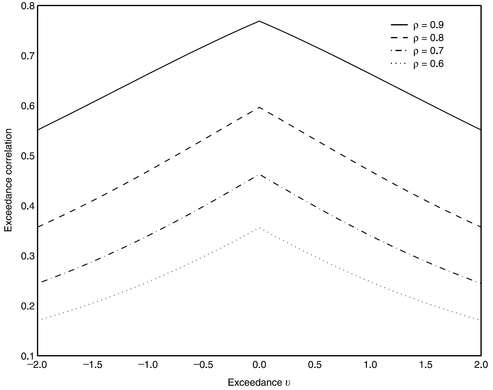You can see how important it is to discuss the correlation structure rather than the average correlation. Even in this canonical, super trivial example, the conditional correlation in either the positive or the negative part of the distribution is lower than that of the unconditional correlation number computed (or reported) based on the full support of both distributions.

Let’s compare the 10% (left) tail conditional correlation between Microsoft stock (MSFT) and the market (SPY). We compute the H-statistic presented in the paper. Intuitively, it will be the excess (conditional) correlation observed in the data over what we should see based on normality assumption. The H-statistic gives us a quantitative measure, since it uses a symmetrical distribution as kind of “benchmark”.


library(quantmod)
library(magrittr)
# citation("quantmod")
k <- 10 # how many years back?
end <- format(Sys.Date(),"%Y-%m-%d")
start <-format(Sys.Date() - (k*365),"%Y-%m-%d")
symetf = c('SPY', 'MSFT')
l <- length(symetf)
w0 <- NULL
for (i in 1:l){
dat0 = getSymbols(symetf[i], src="yahoo", from=start, to=end, 
auto.assign = F, warnings = FALSE,symbol.lookup = F)
	w1 <- dailyReturn(dat0)
	w0 <- cbind(w0, w1)
}
dat <- as.matrix(w0)*100 # percentage
timee <- as.Date(rownames(dat))
colnames(dat) <- symetf
# head(dat)

# install.packages("mvtnorm")
library(mvtnorm)
# citation("mvtnorm")
# Simulate from a bivariate normal with the same first and second moments:
x <- mvtnorm::rmvnorm(n = NROW(dat), mean = colMeans(dat), 
sigma = cov(dat))
# head(x)

quantilee <- 0.1
qspyd <- quantile(x[,"SPY"], quantilee)
qmsftd <- quantile(x[,"MSFT"], quantilee)
# Get a temporary index for the down tail
# When are both in their tail region
tmpindd  <- x[,"SPY"] < qspyd & x[,"MSFT"] < qmsftd
# compute implied by the normal distribution
cor_implied_d <- cor(x[tmpindd,"SPY"], x[tmpindd,"MSFT"])
print(cor_implied_d)
[1] 0.3574835
# Now let's look at the actual data
qspyd <- quantile(dat[,"SPY"], quantilee)
qmsftd <- quantile(dat[,"MSFT"], quantilee)
# Get a temporary index for the down tail
# When are both in their tail region
tmpinddatd  <- dat[,"SPY"] < qspyd & dat[,"MSFT"] < qmsftd
# Compute the observed correlation
cor_obs_d <- cor(dat[tmpinddatd,"SPY"], dat[tmpinddatd,"MSFT"])
print(cor_obs_d)
[1] 0.7325995
# Compute the "magnitude" which cannot be captured 
# by the normal distribution
H_stat <- cor_obs_d - cor_implied_d
print(H_stat)
[1] 0.3751159

library(quantmod)

library(magrittr)

# citation("quantmod")

k <- 10 # how many years back?

end <- format(Sys.Date(),"%Y-%m-%d")

start <-format(Sys.Date() - (k*365),"%Y-%m-%d")

symetf = c('SPY', 'MSFT')

l <- length(symetf)

w0 <- NULL

for (i in 1:l){

dat0 = getSymbols(symetf[i], src="yahoo", from=start, to=end,

auto.assign = F, warnings = FALSE,symbol.lookup = F)

w1 <- dailyReturn(dat0)

w0 <- cbind(w0, w1)

}

dat <- as.matrix(w0)*100 # percentage

timee <- as.Date(rownames(dat))

colnames(dat) <- symetf

# head(dat)

# install.packages("mvtnorm")

library(mvtnorm)

# citation("mvtnorm")

# Simulate from a bivariate normal with the same first and second moments:

x <- mvtnorm::rmvnorm(n = NROW(dat), mean = colMeans(dat),

sigma = cov(dat))

# head(x)

quantilee <- 0.1

qspyd <- quantile(x[,"SPY"], quantilee)

qmsftd <- quantile(x[,"MSFT"], quantilee)

# Get a temporary index for the down tail

# When are both in their tail region

tmpindd <- x[,"SPY"] < qspyd & x[,"MSFT"] < qmsftd

# compute implied by the normal distribution

cor_implied_d <- cor(x[tmpindd,"SPY"], x[tmpindd,"MSFT"])

print(cor_implied_d)

[1] 0.3574835

# Now let's look at the actual data

qspyd <- quantile(dat[,"SPY"], quantilee)

qmsftd <- quantile(dat[,"MSFT"], quantilee)

# Get a temporary index for the down tail

# When are both in their tail region

tmpinddatd <- dat[,"SPY"] < qspyd & dat[,"MSFT"] < qmsftd

# Compute the observed correlation

cor_obs_d <- cor(dat[tmpinddatd,"SPY"], dat[tmpinddatd,"MSFT"])

print(cor_obs_d)

[1] 0.7325995

# Compute the "magnitude" which cannot be captured

# by the normal distribution

H_stat <- cor_obs_d - cor_implied_d

print(H_stat)

[1] 0.3751159

Comments:

This means that 37% are “additional” tail conditional correlation which cannot be accounted for by using a normal bivariate distribution.
You could change the value 0.1 in the line quantilee <- 0.1 to 0.9 to get the 10% upper (right) tail conditional correlation. Given the symmetry of the normal distribution you should get a value which is theoretically the same, but empirically only close to the one for the bottom tail. Then you could compare with what you observe in data as we did here above. This is very similar idea to the proposal I made in my Visualizing tail risk earlier post.
What we did here is to compare what we observe in the data with some canonical model. The paper "asymmetric correlations of equity portfolios" continues to make inference. Rather than compare with some normal distribution, why not create a model which account for the asymmetry and use the H-statistic as an inference tool. It being a difference between data and model, we could accept or reject a model based on how large or small is the H-statistic.

Found this interesting for model-selection and/or portfolio construction.

With my best wishes for the right Stay safe.

References

Ang, Andrew, and Joseph Chen. "Asymmetric correlations of equity portfolios." Journal of financial Economics 63, no. 3 (2002): 443-494. Here for a working-paper version.

TAIL RISK HEDGING