5 weeks ago we took a look at the rising volatility in the (US) equity markets via a time-series threshold model for the VIX. The estimate suggested we are crossing (or crossed) to the more volatile regime. Here, taking somewhat different Hidden Markov Model (HMM) approach we gather more corroboration (few online references at the bottom if you are not familiar with HMM models. The word hidden since the state is ‘invisible’).
We can again use contributed free R-code, the depmixS4 package written by Maarten Speekenbrink and Ingmar Visser who I recently met at the Amsterdam R-meetup group where he gave a talk about the package. RHmm package is another option.
A text book example for estimating Bull-Bear regime switching uses only the return series. However, we can make a sharper model if we add the VIX index as an additional variable which helps to determine the regime. The advantage is that a drawdown can be better classified as being in the bear regime, if it also accompanied by a high levels implied volatility. As oppose to a drawdown which is a natural correction in a bull market.
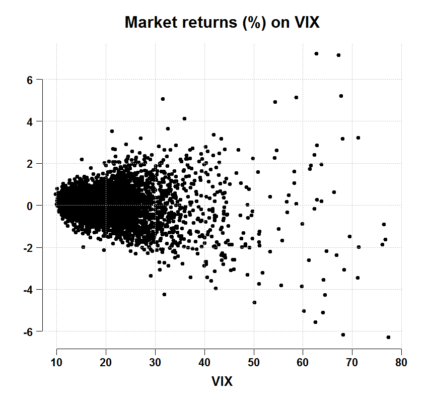
We can see that the biggest moves (thus largest drawdowns) occur when the VIX is high. On the y-axis is the daily returns, on the x-axis is the VIX index in levels:

We estimate the HMM once without the VIX as additional explanatory variable and once with. The equation for the returns in both cases is that they are random-walk (unpredictable), so VIX only enters to the equation which helps determine the state in which we are in. The way it is done is using logistic regression with one of the regimes as ‘base’, so the usual ‘transition matrix’ is not that easy to interpret anymore as in the case where we don’t have any explanatory variables.
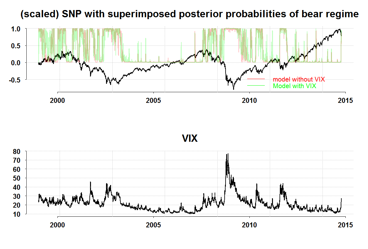
Here is the result, we see (1) a sharper classification with the VIX making sense and (2) oh, we are bear now.
 You can click on the figure for better clarity.
Code for reproduction
|
1 2 3 4 5 6 7 8 9 10 11 12 13 14 15 16 17 18 19 20 21 22 23 24 25 26 27 28 29 30 31 32 33 34 35 36 37 38 39 40 41 42 |
library(TTR) library(depmixS4) library(Eplot) snp <- getYahooData("^GSPC",start=19990101,end=20141016,freq="daily") vix <- getYahooData("^VIX",start=19990101,end=20141016,freq="daily") time <- as.Date(substr(index(snp),1,10))[-1] # get the time index and remove first obs vixp <- apply(vix[,-5],1,mean)[-1] # average daily price (sort of..) # remove first obs # convert to returns (that is why we removed first obs before snpp <- as.numeric(apply(snp[,-5],1,mean)) # average daily price (sort of..) TT <- length(snpp) ret <-100*( snpp[2:TT]/snpp[1:(TT-1)] - 1) # convert to daily returns par(mfrow=c(1,1)) plott(ret,vixp,ret=F,ty="p",xlab="VIX",main="Market returns (%) on VIX") mod <- depmix(ret ~ 1, data=data.frame(ret=ret,vixp=vixp), transition=~1,nstates=2, family=gaussian()) mod2 <- depmix(ret ~ 1, data=data.frame(ret=ret,vixp=vixp), transition=~vixp,nstates=2, family=gaussian()) # mod2 <- depmix(ret ~ vixp, data=data.frame(ret=ret,vixp=vixp), nstates=2) modfit <- fit(mod,verbose=T) modfit2 <- fit(mod2,verbose=T) summary(modfit) summary(modfit2) summary(modfit, which = "transition") summary(modfit2, which = "transition") slotNames(modfit2) trans1 <- as.matrix(posterior(modfit)) trans2 <- as.matrix(posterior(modfit2)) ## The Figure par(mfrow=c(2,1)) col1 <- rgb(1,0,0,1/4) col2 <- rgb(0,1,0,1/4) par(mfrow=c(2,1)) plott(scale(snpp[-1],scale=T)/3,time,ret=F,ty="l",main="(scaled) SNP with superimposed posterior probabilities of bear regime") plott(trans1[,2],time,ty="l",ret=F,col=col1,add=T) plott(trans2[,3],time,ty="l",add=T,col=col2) # the other regime is base legend('bottomright',legend=c("model without VIX","Model with VIX"),cex=1.3, col=c("red","green"),lty=1,bty="n",text.col=c("red","green")) plott(vixp,time,ty="l",main="VIX") |
References:
http://petewerner.blogspot.nl/2014/09/hmm-example-with-depmixs4.html
http://gekkoquant.com/2014/09/07/hidden-markov-models-examples-in-r-part-3-of-4/ http://econweb.ucsd.edu/~jhamilto/handbook_regimes.pdf
[asa onelinertpl]0898716659[/asa]


It would be interesting to see the equity curve of the periods without the bear mode triggered. I think it would show great returns.
When calling posterior(modfit), why can there be “State = 1” even if S2 Probability is >90%? Thank you! Felix