What is a Latent Variable?

This post provides an intuitive explanation for the term Latent Variable.

Assume this is your realization of the data:

Realization of a bivariate distribution

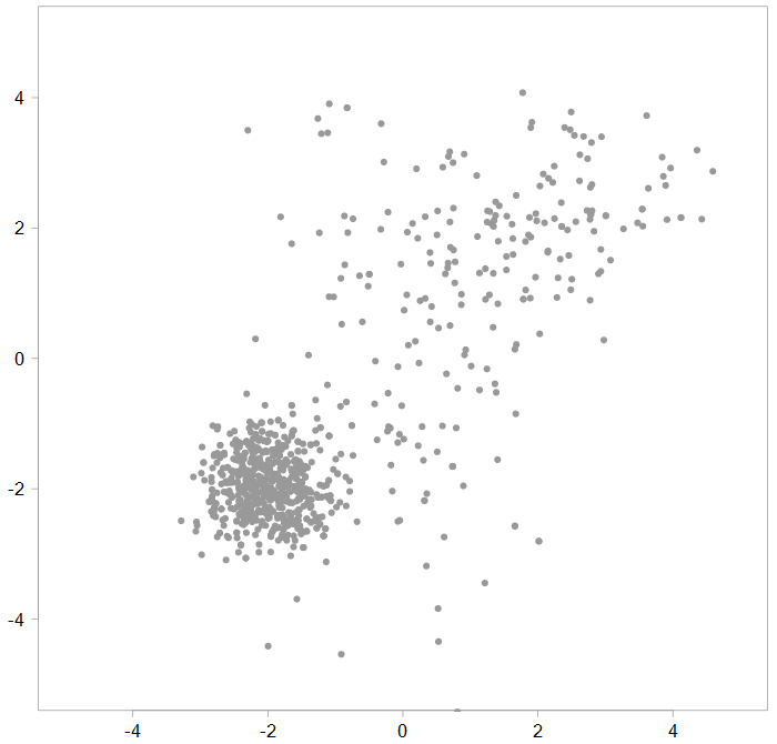
Now you try to figure out where this data is coming from, what is the underlying generating process. It looks like a non-standard joint distribution, so you decide to describe it as a mixture of distributions (Mixture Models reference). Spoiler alert: the data is indeed generated by a mixture of three Gaussian distributions. From here onward we refer to those individual distributions as components and reserve the word distribution for the overall (mixture) distribution.

A mixture of three bivariate components

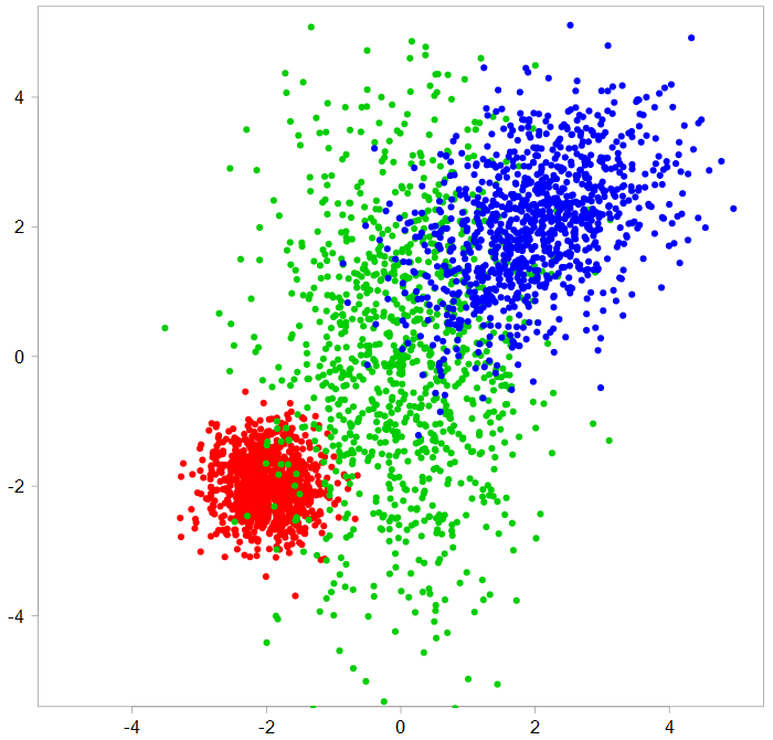
You can see that each component has its own mean vector and covariance matrix, which are different (code below). In reality you only see the first grey chart above, so you have no idea how many underlying components and what they look like.

So what is a Latent Variable?

The word latent means hidden. So a latent variable is one that matters, but we can’t see it. In this case it is the proportion that comes from each component. The way the data was generated is such that the first component (in red) had much higher proportion (75%) than the other two (12.5% each). Exactly what was the split between the three components can only be inferred, not observed. Hence the name.

Wait wait wait, but we can’t also observe the mean and covariance of each components, those we also can only be inferred, but we don’t call those latent variables right? Right, and here’s why.

The term variable is so often used that we tend to forget- not unlike we tend to forget what is printed on a 5 Euros note which is also often used- that it is variable. The mean and covariance are unknown parameters, but they are not changing\variable. When we draw an observation from the mixture distribution above, it actually depends on a random variable with a categorical distribution: , for i which is first, second or third component.

In our case p(x=1) = 0.75, which created the figure about, because each time we draw an observation, it had 75% chance of having a first component’s mean and covariance. However, if the realization would look like so:

Different realization of a bivariate distribution

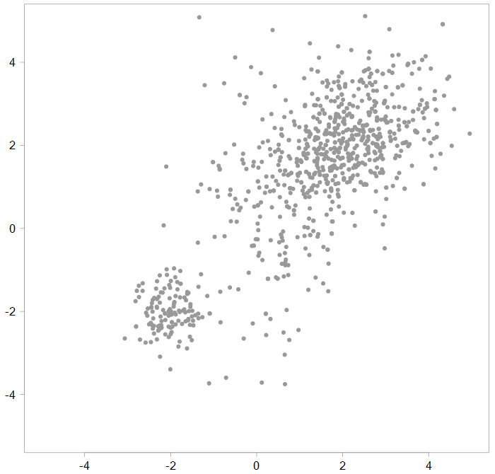Then we would estimate that the latent variable may have a p(x=1) = p(x=2) = 0.125, and p(x=3) = 0.75, rather.

There are other examples for latent variables, but this is a very common one schematic example.

Code and References

An R Package for Analyzing Finite Mixture Models

Finite Mixture and Markov Switching Models