As the title reads, few more R-related tips and tricks. I hope you have not seen those before.
Some utilities
Methods are functions which are specifically written for particular class. In the post Show yourself (look “under the hood” of a function in R) we saw how to get the methods that go with a particular class. Now there are more modern, less clunky ways for this.
See which methods are available per class
Have a look at the sloop package, maintained by Hadley Wickham (that alone is a reason). Use the function s3_methods_generic to get a nice table with some relevant information:
|
1 2 3 4 5 6 7 8 9 10 11 12 13 14 15 16 17 18 19 20 |
# install.packages("sloop") library(sloop) citation("sloop") s3_methods_generic("mean") # s3_methods_generic("as.data.frame") # A tibble: 10 x 4 generic class visible source <chr> <chr> <lgl> <chr> 1 mean Date TRUE base 2 mean default TRUE base 3 mean difftime TRUE base 4 mean POSIXct TRUE base 5 mean POSIXlt TRUE base 6 mean quosure FALSE registered S3method 7 mean vctrs_vctr FALSE registered S3method 8 mean yearmon FALSE registered S3method 9 mean yearqtr FALSE registered S3method 10 mean zoo FALSE registered S3method |
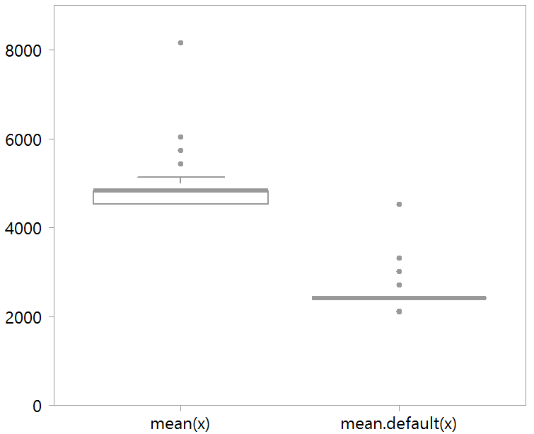
You can use the above to check if there exists a method for the class you are working with. If there is, you can help R by specifying that method directly. Do that and you gain, sometimes meaningfully so, a speed advantage. Let’s see how it works in couple of toy cases. One with a Date class and one with a numeric class.
|
1 2 3 4 5 6 7 8 9 10 11 12 13 14 15 16 17 18 19 20 21 22 23 24 25 26 27 28 |
library(magrittr) # for the piping operator # install.packages("scales") # we talk about this shortly library(scales) # install.packages("microbenchmark") library(microbenchmark) citation("microbenchmark") # Create a sequence of dates some_dates <- seq(as.Date("2000/1/1"), by = "month", length.out = 60) bench <- microbenchmark(mean(some_dates), mean.Date(some_dates), times = 10^3) %>% summary print(bench) expr min lq mean median uq max neval 1 mean(some_dates) 6.038 6.642 7.011879 6.642 6.944 14.189 1000 2 mean.Date(some_dates) 4.528 4.831 5.417070 5.133 5.435 51.923 1000 cat("Save", (1 - bench$mean[2] / bench$mean[1]) %>% percent(digits = 2)) Save 23% # Now something more standard x <- runif(1000) # simulate 1000 from random uniform bench <- microbenchmark( mean(x), mean.default(x) ) print(bench) expr min lq mean median uq max neval 1 mean(x) 4.529 5.133 7.113611 7.548 8.453 44.376 1000 2 mean.default(x) 2.113 2.416 3.148788 3.321 3.623 9.963 1000 > cat("Save", (1 - bench$mean[2] / bench$mean[1]) %>% percent(digits = 2)) Save 56% |
Specifying the exact method (if it is there) also reduces the variance around computational time, which is important for simulation exercises:

Percent formatting
In the code snippet above I used the scales package’s percent function, which spares the formatting annoyance.
Get your object’s size
When I load a data, I often want to know how big is it. There is the basic object.size function but it’s ummm, ugly. Use the aptly named object_size function from the pryr package.
|
1 2 3 4 5 6 7 8 9 10 11 12 13 14 15 16 17 18 19 20 21 22 23 24 |
library(pryr) citation("pryr") > x <- runif(10^3) > object_size(x) 8.05 kB > object.size(x) 8048 bytes > x <- runif(10^6) > object_size(x) 8 MB > object.size(x) 8000048 bytes > x <- runif(10^8) > object_size(x) 800 MB > object.size(x) 800000048 bytes # is this Mega or Giga? > x <- runif(10^9) > object_size(x) 8 GB > object.size(x) 8000000048 bytes # is this Mega or Giga? |
Memory management
Use the gc function; gc stands for garbage collection. It frees up memory by, well, collecting garbage objects from your workspace and trashing them. I at least, need to do this often.
heta function
I use the head and tail functions a lot, often as the first thing I do. Just eyeballing few lines helps to get a feel for the data. Default printing parameter for those function is 6 (lines) which is too much in my opinion. Also, especially with time series data you have a bunch of missing values at the start, or at the end of the time frame. So that I don’t need to run each time two function separately, I combined them into one:
|
1 2 3 4 5 6 7 8 |
heta <- function(x, k= 3){ cat("Head -- ","\n", "~~~~~", "\n") print(head(x, k)) cat("Tail -- ","\n", "~~~~~", "\n") print(tail(x, k)) } |
Sound the alarm
If you stretch your model enough, you will have to wait until computation is done with. It is nice to get a sound notification for when you can continue working. A terrific way to do that is using the beepr package.
# install.packages("beepr")

library(beepr)

citation("beepr")

for (i in 0:forever){

do many tiny calculations and don't ever converge

}

beep(4)
Click play to play:
Enjoy!


