In the last decade we have observed an increase in computational power, information availability, speed of execution and stock market competition in general. One might think that, as a result, we are prone to larger shocks that occur faster than what was common in the past. I crunched some numbers and was surprised to see that this is not the case.
We can use the Kurtosis as a proxy for extreme events, high Kurtosis in a certain month means that the return distribution for that month was such that most observations were in the center, and some were in the tails, the higher the kurtosis, the fatter the tail. Here I do not differentiate between positive and negative shocks.
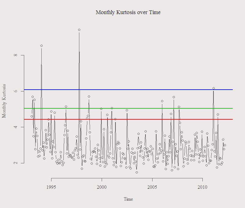
Here is a figure of the monthly Kurtosis, calculated from the S&P returns, over time, starting from 1993 until 2012. The Lines correspond with the 90%,95% and 99% quantiles of the series.
 We can see that this measure is quite steady over time with a few jumps that correspond with past extreme events. No upward trend is observed and the number of months with very high Kurtosis do not appear to be more likely nowdays than in the past. This means that you can prepare yourself before losing your money as oppose to just wake up to see your account, which was just fine the night before, now needs more collateral.
Note:
We should not really care about the right tail when we calculate risk (if we are long that is). You can also try this exercise with Semi-Kurtosis, call it partial moment for academic ambiguity. The positive side will represent “potential upward jumps” while the denominator (negative side) will counter that with “potential train through your stomach”.
Related:
Probable Outcomes: Secular Stock Market Insights
Unexpected Returns
Expected Returns
Code:
|
1 2 3 4 5 6 7 8 9 10 11 12 13 14 15 16 17 18 19 20 21 22 |
library(quantmod) ; library(e1071) tckr = c('SPY') # the ETF on the S&P end<- format(Sys.Date(),"%Y-%m-%d") # yyyy-mm-dd start<-format(Sys.Date() - 365*20,"%Y-%m-%d") dat1 = (getSymbols(tckr[1], src="yahoo", from=start, to=end, auto.assign = FALSE)) ret1 = as.numeric((dat1[,4] - dat1[,1])/dat1[,1] ) n = length(as.numeric(ret1)) time0 = index(dat1) head(time0) ; tail(time0) s = seq(1,n,22) # make it monthly k = NULL for (i in 1:(length(s)-1)){ k[i] = 3+kurtosis(ret1[s[i]:s[(i+1)]]) } time0[s[which(k>quantile(k,.95))]] # which months plot(k~time0[s[1:(length(s)-1)] ], ty = "b", xlab = "Time", ylab = "Monthly Kurtosis", main = "Monthly Kurtosis over Time") abline(a = quantile(k,.90), b = 0, lwd = 2, col = 2) abline(a = quantile(k,.95), b = 0, lwd = 2, col = 3) abline(a = quantile(k,.99), b = 0, lwd = 2, col = 4) |


In the code shown above, you seem to have taken the intraday return (close-open) for calculating the kurtosis for the month. Is this intentional and do we have to use that to calculate kurtosis? Or should we use the traditional close-close return for this?
Thanks.
Your question is good. I trade intra-day, so I naturally care more about the intra-day move (position is only open during trading hours). For over night positions it would indeed be better to use the more standard Close to Close and take it from there. Thanks for the comment.