Understanding Word Embeddings (2)

I have noticed that when I use the term “coordinates” to talk about vectors, it doesn’t always click for everyone in the room. The previous post covered the algebra of word embeddings and now we explain why you should think about the vector of the word embedding simply as coordinates in space. We skip the trivial 1D and 2D cases since they are straightforward. 4 dimensions is too complicated for me to gif around with, so 3D dimensions would have to suffice for our illustrations.

Geometric interpretation of a word embedding

Take a look at this basic matrix:

$\begin{array}{c|ccc} & \text{dog} & \text{cat} & \text{fish} \\ \hline \text{word}_1 & 1 & 0 & 0 \\ \text{word}_2 & 0 & 1 & 0 \\ \text{word}_3 & 0 & 0 & 1 \end{array}$

The one-hot word-vectors are visualized in the 3D space as follows:

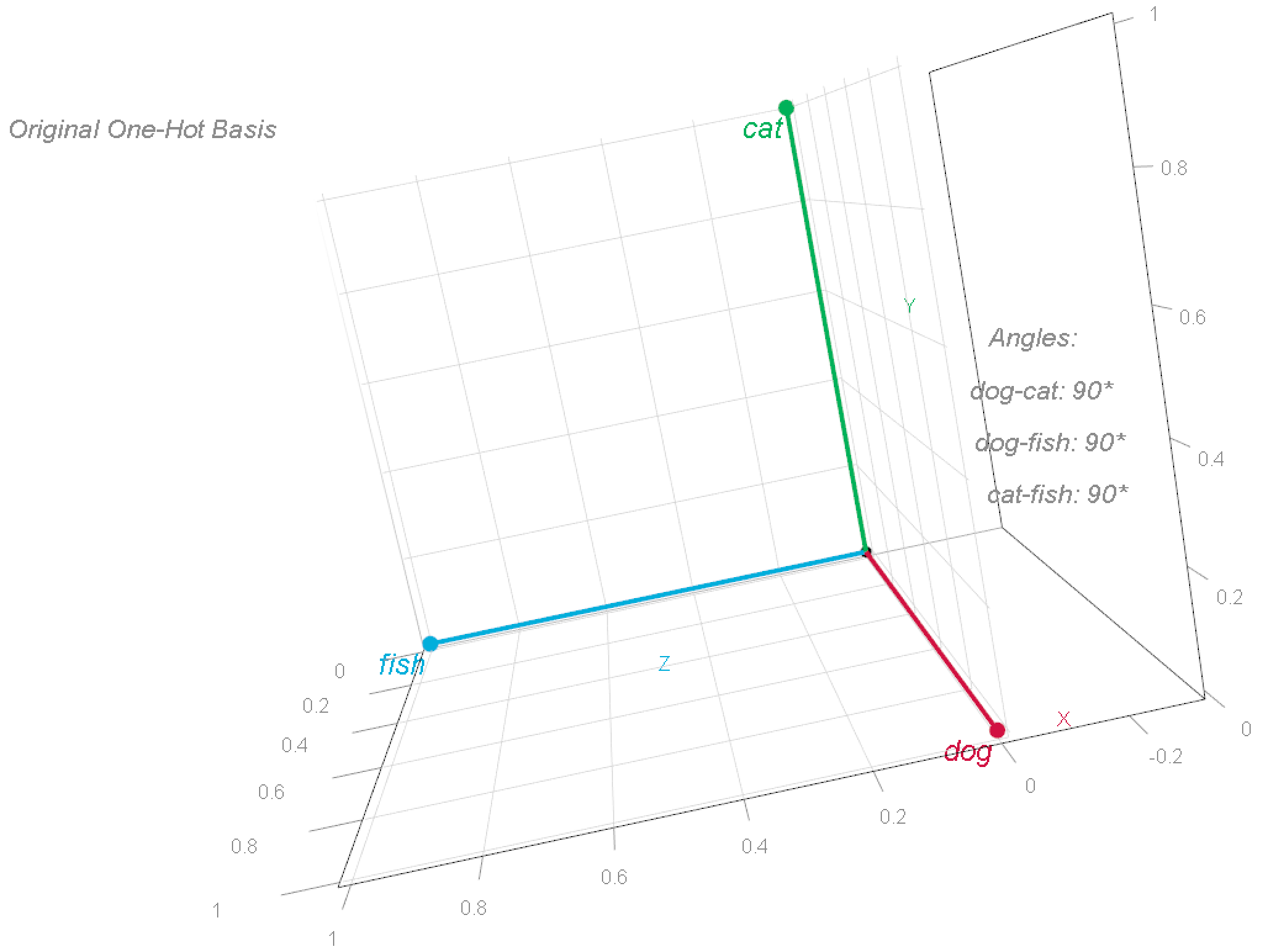
To better understand this coordinate system, we can rotate these vectors. This changes the words’ coordinates, but preserves their relationships—specifically, the angles between them remains at 90°.

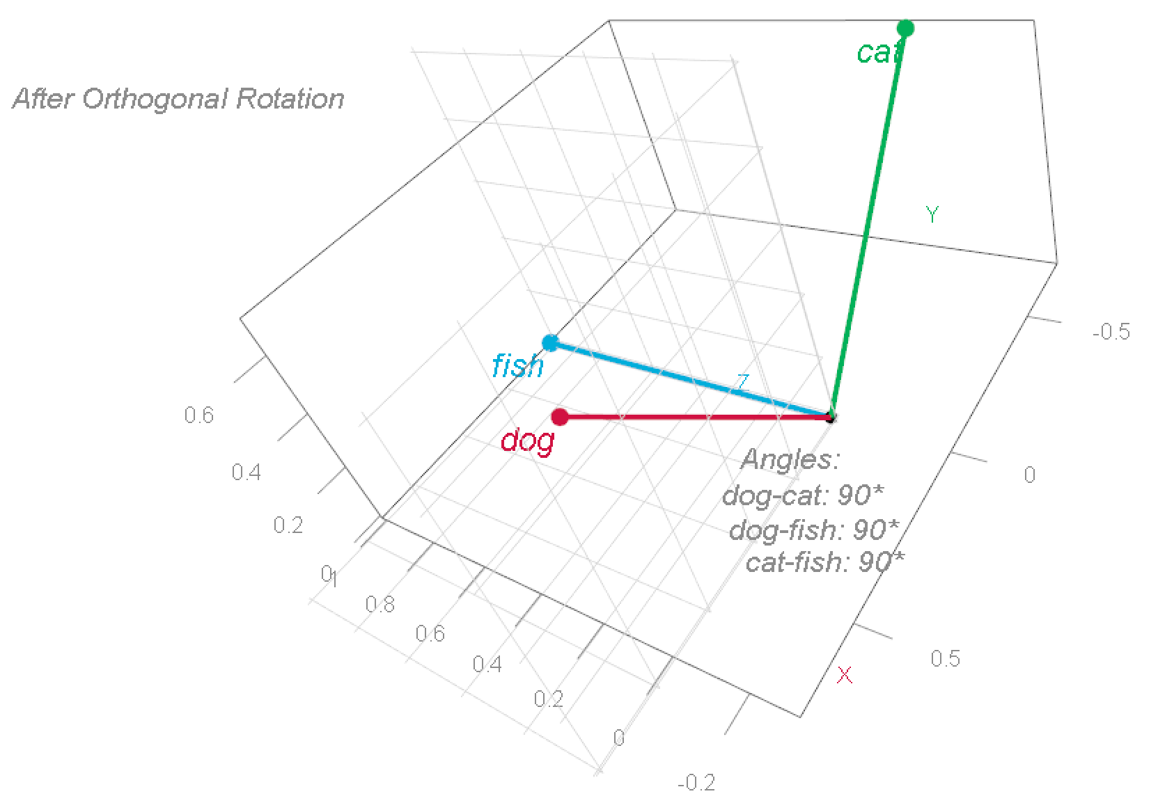
Observe that he word fish remained where it was, the word cat now sits at [-0.707, 0.707, 0] and the word dog sits at [0.707, 0.707, 0], but the relationship between the words has not changed (it’s a 3d image, the angles are still 90° apart). This illustrates a specific example for what is called “basis transformation” (the term “basis” is explained in the previous post).

Basis transformation in our context of word embeddings means that we change our rudimentary one-hot representation, where words are represented in the standard basis, to the embedding representation where words are represented in a semantic basis.

Semantic basis 🤨 ? Yes, let me explain. Semantics is the branch of linguistics and logic concerned with meaning. But, “meaning” is a latent and ill-defined concept. There are different ways to describe what one means: both “inflation” and “rising-prices” map to almost identical meaning. Related to that, a frequent misconception in the field of NLP topic modeling is the belief that topics are actually-defined things, which they are not. In fact, we might consider ourselves fortunate if a topic can even indirectly be inferred from the words assigned to the same cluster (e.g., “topic 3”). For instance, if words like deflation, stagflation, and inflation appear together in the same cluster, we could interpret that cluster as “price stability” topic – even if, as it happens, the cluster also includes many other, unrelated, words. So when we refer to semantics, we’re basically talking about the underlying, unobserved\abstract\latent and ill-defined term: meaning.

What makes a space semantic is how words connect to each other. That’s different from the example above where each word just stands on its own – ‘cat’ doesn’t have any special relationship to ‘dog’ or ‘fish’, all three words are alone standing.

So that we understand the term “semantic”, let’s see what is gained by shifting from our clear and precise one-hot encoding space, to a semantic space.

Word Coordinates in Semantic Space

Semantic space is better than a formal/symbolic/non-semantic space largely due to these two advantages:

Dimension reduction (we save storage- and computational costs).
We can relate words to each other. It’s beneficial if words like revenues and earnings aren’t entirely independent algebraically, because in reality they are not independent in what they mean for us (e.g. both words imply to potentially higher profits).

Unpacking in progress:

Dimension reduction: In one-hot word-representation each word is completely distinct (all 90°, i.e. independent). Words share no common components and are completely dissimilar (similarity=0) in that representation. The upside is that we capture all words in our vocabulary and each word has a clear specific location. But, that space is massive: each vector is of size equals to the number of unique words (vocabulary). When we embed word-vectors we cast each word-vector into a lower dimension space. Instead of a coordinate system with $V$ dimensions, we use a lower-dimension coordinate system, say 768. Now each word will not be where it should be exactly. Why not? because we don’t have $V$ entries to place that word in space, we only have 768, so each word will be placed somewhere inside our 768 coordinate system. By compressing all those $V$ words into just 768 dimensions, we produce a denser representations instead of the extremely sparse one-hot vectors. We inevitably lose the independence that one-hot encodings provided, but this also presents an opportunity to compress the $V$ words in a way that places related words closer together in the compressed 768 dimensional space.
We can relate words to each other: For the following dense word-vectors representation (being silent for now about how to find these vectors)

$\begin{pmatrix} \text{dog:} & 0.8 & 0.2 & 0.3 \\ \text{cat:} & 0.7 & 0.3 & 0.4 \\ \text{fish:} & 0.1 & 0.9 & 0.2 \end{pmatrix}$

The plot below shows ‘cat’ and ‘dog’ are spatially closer, indicating their greater semantic similarity compared to their similarity with ‘fish’.

I won’t get into the details of how we find these dense word-vectors. The short version is that we some transformer model to create those vectors for us. The transformers family of models has the great power to, well.. transform an initial and imprecise, a guess if you will, set of coordinates (word-vectors), into a much more reasonable one. Reasonable in that words eventually end up placed near other words that relate to them (think back to our ‘revenues’ and ‘earnings’ example).

Note that we did not demonstrate dimension reduction here (the representation stayed in 3 dimensions), this illustration focused only on the acquisition of meaning.

To exemplify dimension reduction we could can map the three vectors into a 2 dimensional space: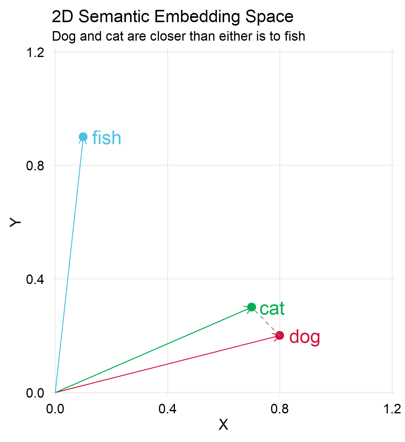

As mentioned, dimension reduction helps reduce storage and compute costs, but do we lose anything? Absolutely we do.

The Crowding Problem

Notice that in the 3d space, our one-hot basis can be placed such that all vectors are perpendicular to each other. This is not possible in a 2d space. But we deliberately chose a projection that maintains key distinctions, in our simple example: keeping “dog” and “cat” close to each other while “fish” is distant. What about higher dimensions?

When reducing dimensionality from the exact one-hot space, with the number of vectors in the hundreds of thousands, to a smaller space, say 768 dimensions, we distort our representation, call it compression costs. Simply put, half a million points, once living large, now have to cram into a cheap dorms, with some tokens snoring more than others. This compression-induced distortion is known by the evocative term ‘the crowding problem’. You may have wondered (I know I did) why do we stop at fairly moderate dimensions? Early language models had dimensions of 128, then 512, 768, 1024, 3072 and recently 4096 and that’s about it. Don’t we gain better accuracy if we use say $10^4$ ?

We don’t. Enter the Johnson-Lindenstrauss (JL) Lemma.

The Johnson-Lindenstrauss (JL) Lemma

One variation of the lemma is:
Let $0 < \varepsilon < 1$ , and let $X \subset \mathbb{R}^n$ be a set of $n$ points. Then, for any integer $k \geq \frac{4 \ln n}{\varepsilon^2}$ , there exists a linear map $f: \mathbb{R}^n \rightarrow \mathbb{R}^k$ such that for all $a, b \in X$ :

$(1 - \varepsilon) \|a - b\|^2 \leq \|f(a) - f(b)\|^2 \leq (1 + \varepsilon) \|a - b\|^2,$

where $f$ is The function that maps points from high-dimensional space to low-dimensional space. $f(a), f(b)$ are the projections of points $a$ and $b$ in the lower-dimensional space. Specifically $f(x) = Rx$ where $R$ is the projection matrix. If you are reading this you probably know what PCA is, so think about $R$ as the rotation matrix; to find the first few factors you need to multiply the original variables with the first few rotation-vectors. $||\cdot||$ is the Euclidean norm (squared distance), and finally $\varepsilon$ is the distortion parameter (typically between 0 and 1).

Simply speaking, the JL lemma states that a set of $n$ points, a point in our context is a word-vector, in high-dimensional space can be mapped into a space of dimension $O\left(\frac{\log n}{\varepsilon^2}\right)$ (much lower than $n$ ..) while still preserving pairwise distances up to a factor of $(1 \pm \varepsilon)$ . As an example, 100,000 points (vocabulary of 100,000) can be theoretically mapped to

$\frac{log_2(100,000) \approx 17}{0.1^2} \approx 1700.$

Setting $\varepsilon = 0.1$ means that we accept a distortion of 10%; so if the original distance between vector $a$ and vector $b$ is $d$ , then after the compression it will be between $0.9d$ and $1.1d$ .

Remarks:

Fun fact: in sufficiently large dimension even random projection – where $f(x) = RX$ , with the vectors of $R$ simply drawn randomly, also approximately preserves pairwise distances. You can (should) compress large dimensional data without carefully engineering $R$ , for example you don’t always have to spend time doing singular value decomposition. I leave it for the curious reader to check this counter-intuitive fact.
As typical data are, most of the structure is often captured by the first few dimensions. Again, you can think about the first few factors as capturing most of the variation in the data. Adding factors beyond a certain point can add value, but with sharply diminishing returns. Another fun fact (perhaps I should rethink my perception of fun 🥴), you capture most of the variation with the first few dimensions even if the data is completely random (meaning no structure to be captured whatsoever). This fact was flagged recently in the prestigious Econometrica journal as spurious factors (looks like a factor but simply the result of the numerical procedure).
As oppose to the curse of dimensionality, we can think of the ability to compress high-dimensional data without losing much information as the blessing of dimensionality, because it’s simply the flip side of the curse. It cuts both ways: it’s fairly easy to shrink high-dimensional spaces down because points in that space are so spread-out, which is exactly why finding meaningful patterns in high-dimensional space is such a headache to begin with.

In sum

We moved from one-hot representation of words in a high-dimensional space to a lower-dimensional “semantic space” where word relationships are captured. We showed how word vectors can be rotated without changing their relative positions. This transformation is crucial because it allows us to represent word meaning and relationships, reducing storage and computation costs. We then moved on to the “crowding problem” that arises from dimensionality reduction and introduced the Johnson-Lindenstrauss (JL) Lemma, which provides the theoretical legitimacy for compressing high-dimensional text data.

I hope you now have a better grip on:

Why we can refer to word-vectors as coordinates in space

Why it’s ok to do, and why we don’t lose much information about word relationships

Together with the previous post providing the algebraic foundation for word-embeddings you are well-positioned to, actually understand, transformers and LLMs better.