Laws of large numbers

The laws of large numbers are the cornerstones of asymptotic theory. ‘Large numbers’ in this context does not refer to the value of the numbers we are dealing with, rather, it refers to a large number of repetitions (or trials, or experiments, or iterations). This post takes a stab at explaining the difference between the strong law of large numbers (SLLN) and the weak law of large numbers (WLLN). I think it is important, not amply clear to most, and I will need it as a reference in future posts.

Before we go to the actual laws, lets first differentiate between strong convergence and weak convergence.

Strong would mean that at the limit, you know the number exactly; we call it ‘almost surely’ for reasons too weighty for us here (measure theory).

Weak would mean that you would only know the limit approximately, but also that you can have as good approximation as you want, but never (ever) the number exactly. This is the main origin for the head–scratching: if you can get as close as you want, why can’t you, then, exactly determine the number? follow me.

Strong law of large numbers

Strong convergence. The sample average converges (almost surely) to the expected value. Formally:

(1) $\begin{equation*} \bar{X}_n\ \xrightarrow{\text{a.s.}}\ \mu \qquad\textrm{when}\ n \to \infty, \end{equation*}$

while $\bar{X}_n$ is simply the average which is based on $n$ observations. This is the same as saying that at the limit, you know what the average is (based on infinite amount of observations, it is the expected value) with probability one:

(2) $\begin{equation*} \Pr\!\left( \lim_{n\to\infty}\bar{X}_n = \mu \right) = 1. \end{equation*}$

Strong law of large numbers – illustration

Let’s simulate from normal distribution, and compute the average at each point in time.


NN <- 10000
x <- rnorm(NN)
seq_sum <- NULL
for(i in 1:NN){
  seq_sum[i] <- sum(x[1:i])/i
}

NN <- 10000

x <- rnorm(NN)

seq_sum <- NULL

for(i in 1:NN){

seq_sum[i] <- sum(x[1:i])/i

}

Now let’s plot it:

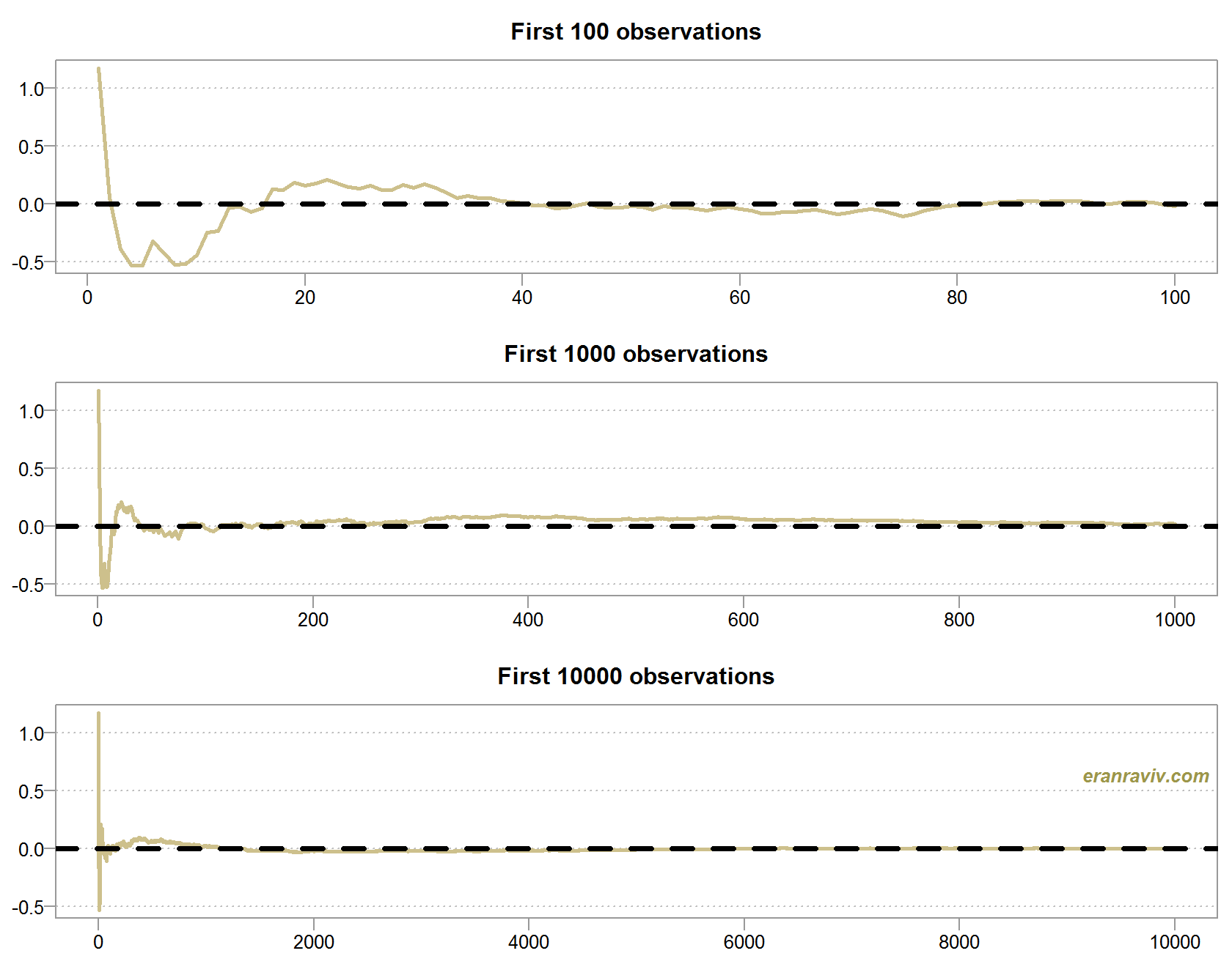
Strong law of large numbers demonstration

As you can see, the larger the n, the closer the average to the mean, which is zero in this illustration. Strong, or almost-sure convergence means that as some point, adding more observation does not matter at all for the average, it would be exactly equal to the expected value.

Weak law of large numbers

(3) $\begin{equation*} \overline{X}_n\ \xrightarrow{P}\ \mu \qquad\textrm{when}\ n \to \infty. \end{equation*}$

Note instead of the $a.s$ above the arrow, which stands for almost surely, we now have $P$ which indicates weak convergence, or convergence in probability. Recall what we already mentioned, that we get as good approximation as we would like to. That is to say that for any positive number $\varepsilon$ ,

(4) $\begin{equation*} \lim_{n\to\infty}\Pr\!\left(\,|\overline{X}_n-\mu| > \varepsilon\,\right) = 0. \end{equation*}$

In words, the probability that the average is “far” from the mean $\mu$ more than that (arbitrary) number $\varepsilon$ , is zero. But that number is positive, as small as we want but it is there smirking nonetheless.

Weak law of large numbers – illustration

Say x is a random variable from exponential distribution with rate parameter $\lambda=1$ . Now consider the quantity

$\frac{\sin(x)}{x}$

with expected value:

(5) $\begin{equation*} E\left(\frac{\sin(x)}{x}\right) = 0 \end{equation*}$


g <- rexp(NN)
seq_sum_exp <- NULL
for(i in 1:NN){
  seq_sum_exp[i] <- sum( (sin(g[i]) )/g[i] )  /  i
}

g <- rexp(NN)

seq_sum_exp <- NULL

for(i in 1:NN){

seq_sum_exp[i] <- sum( (sin(g[i]) )/g[i] ) / i

}

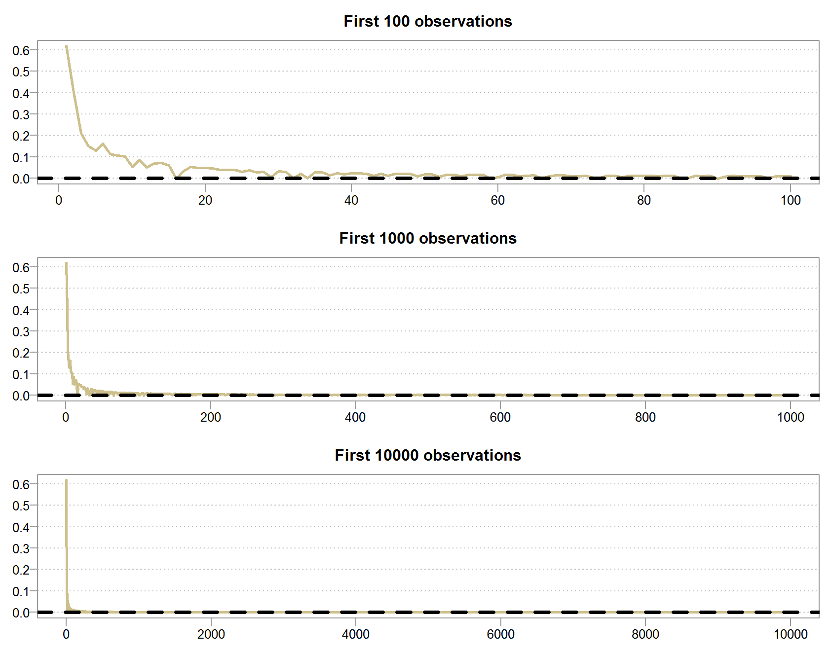
Looks fairly similar to the previous illustration doesn’t it? But it is different.

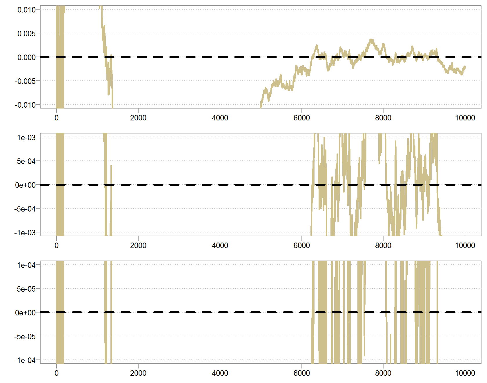
Zooming in

Lets take a closer look at the series. Zoom in slowly so we can see how the series behave closer to the expectation.
The Y axis is tighter and tighter from top to bottom panel.

Strong law of large numbers demonstration (zoom)

We see that the series is not close to zero, most of the time, but is quite smooth in that when it is closer to zero, it tends to stay close for some time. It is already creeping back to zero and from the behavior it is easy to imagine that at some point it will simply hoover closer and closer, and closer, without deviating at all anymore. The ‘smoothness’ of this series would make it impossible for a single observation to pull the series away from the average at the limit.

In contrast, lets plot the other series in the same way:

Weak law of large numbers demonstration (zoom)

Here we see a different behavior. Because $x \sim exponentially,$ there is always a chance that we draw an observation which is very close to zero, and so always a chance to get a very large number which will push the series astray from its mean. Look at the white space between the lines, despite the fact that it is harder and harder to push the series away from the mean, the frequency in which that happens is somewhat constant. So maybe the series will be closer and closer to zero, but because the frequency is constant, and not decreasing as for the other series, we will never be exactly at zero.

To clarify this, we can simulate some observation from a random exponential variable:

Few observations from exponential distribution

The point is that there is always a positive, non-vanishing chance for a number which is as close to zero as to still be able to push the average astray, for whichever $n$ you have.

Few more comments

The Weak is weak because if the Strong holds, the Weak follows, but not the reverse. If you are reading these final lines then this statement probably does not require any more explanations. When reading proofs I most often encounter convergence of the Strong form. There is another type of convergence which is called convergence in distribution, where instead of converging to a constant, we converge to a random variable which has some distribution. But that’s for another time.