A way to think about principal component analysis is as a matrix approximation. We have a matrix  and we want to get a ‘smaller’ matrix
  with
with  . We want the new ‘smaller’ matrix to be close to the original despite its reduced dimension. Sometimes we say ‘such that Z capture the bulk of comovement in X. Big data technology is such that nowadays the number of cross sectional units (number of columns in X) P has grown to be very large compared to the sixties say. Now, with ‘google maps would like to use your current location’ and future ‘google fridge would like to access your amazon shopping list’, you can count on P growing exponentially, we are just getting started. A lot of effort goes into this line of research, and with great leaps.
In OLS, the objective is to minimize  . In our case we have no fitted values since we have no Y, we want to approximate X to itself in a smart way. We create “
 ” and call those the factors. That is also the reason for identifiably issues, and we always write that some more restrictions are needed. When you have only the X, this guy:
  can be created using many combinations of Y and the coefficients, you can’t determine both in a unique manner.
Most common way to establish the factors is via spectral decomposition. Lets construct the factors for some basic ETF’s. Easily in R :
|
1 2 3 4 5 6 7 8 9 10 11 12 13 14 15 16 17 18 19 20 21 22 23 24 25 26 27 28 29 |
library(quantmod) sym = c('IEF','TLT','SPY','QQQ') l=length(sym) end<- format(Sys.Date(),"%Y-%m-%d") start<-format(as.Date("2007-01-01"),"%Y-%m-%d") dat0 = (getSymbols(sym[1], src="yahoo", from=start, to=end, auto.assign = F)) n = NROW(dat0) dat = array(dim = c(n,6,l)) ; prlev = matrix(nrow = n, ncol = l) for (i in 1:l){ dat0 = (getSymbols(sym[i], src="yahoo", from=start, to=end, auto.assign = F)) dat[1:length(dat0[,1]),,i] = dat0 # Average Price during the day prlev[1:length(dat0[,1]),i] = as.numeric(dat[,4,i]+dat[,1,i]+dat[,2,i]+dat[,3,i])/4 } time <- index(dat0) par(mfrow = c(2,2)) x <- prlev # only change of name mean_prlev <- apply(prlev,1,mean) # for plotting TT <- dim(x)[1];TT p <- NCOL(x) pc0 <- prcomp(x,center=T,scale=T) # plot par(mfrow = c(2,1),bg='azure2') matplot(x,ty="l",pch=1:p,main="Bold is the first PC",ylab="") lines(pc0$x[,1]+mean_prlev,lwd=7,col=1) legend('topleft',sym,lty=1:p,col=1:p,bty='n',ncol=2) barplot(pc0$rot[,1],names.arg=sym,main='loadings on First PC') |
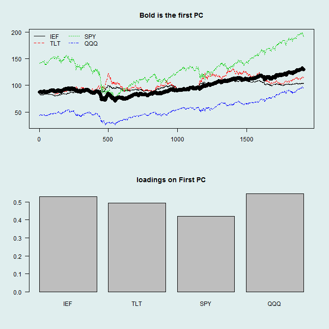
In general, we should not do this using non-stationary series, but for illustration it is better. The bold line is the first column from the approximated matrix
( ). As you can see from the loadings, it is pretty much the average of the other four columns which is typical. To better understand what R is doing we can do the decomposition ourselves. Formally, the loadings are the eigenvectors corresponding to the K largest eigenvalues of the
  , which is the covariance (or correlation when scaled) of X up to a constant.
|
1 2 3 4 5 6 7 8 9 10 11 12 13 14 15 16 17 |
> sx <- scale(x,scale=T) > xxprime = t(sx)%*%(sx) > eigval = eigen(xxprime,symmetric=T) > eigval$vectors [,1] [,2] [,3] [,4] [1,] -0.5282730 0.4297762 0.4433804 0.5827812 [2,] -0.4945851 0.5038988 -0.6140131 -0.3527882 [3,] -0.4212469 -0.6523735 -0.4496436 0.4413395 [4,] -0.5466847 -0.3684933 0.4735213 -0.5840600 > pc0$rot PC1 PC2 PC3 PC4 [1,] 0.5282730 -0.4297762 0.4433804 -0.5827812 [2,] 0.4945851 -0.5038988 -0.6140131 0.3527882 [3,] 0.4212469 0.6523735 -0.4496436 -0.4413395 [4,] 0.5466847 0.3684933 0.4735213 0.5840600 |
Coming back to the OLS way of thinking, naturally, these loadings are the same as what we get if we project the factors onto the X space:
|
1 2 3 4 5 6 7 8 9 10 11 12 |
cof <- matrix(nrow=p,ncol=p) for (i in 1:p){ cof[,i] <- lm(pc0$x[,i]~0+sx)$coef } cof [,1] [,2] [,3] [,4] [1,] 0.5282730 -0.4297762 0.4433804 -0.5827812 [2,] 0.4945851 -0.5038988 -0.6140131 0.3527882 [3,] 0.4212469 0.6523735 -0.4496436 -0.4413395 [4,] 0.5466847 0.3684933 0.4735213 0.5840600 |
This regression-like style is now becoming more and more relevant. When P is very large relative to T, the procedure is not stable. Following this line of thinking, we can utilize all the tools from regression literature, i.e. ridge regression and LASSO, to stabilize the loading matrix using shrinkage.


Interesting way of thinking about it. Nice article!
how would one go about doing a pca regression in R in your above example?
PCA Regression (PCR) is different. You first ‘condense’ the information in your X matrix using PCA and use the first few (say first 5) principal component as regressors.