Local Linear Forests

Random forests is one of the most powerful pure-prediction algorithms; immensely popular with modern statisticians. Despite the potent performance, improvements to the basic random forests algorithm are still possible. One such improvement is put forward in a recent paper called Local Linear Forests which I review in this post. To enjoy the read you need to be already familiar with the basic version of random forests.

The result of a random forest can be thought of as an average over many predictions arising from individual trees – quite intuitive. For this post we need a companion view to random forest. In order to understand where and why improvement to random forest is possible I start by providing a complementing intuition and different formulation of the random forest algorithm.

The traditional view of random forest is:

$\hat{f}\left(x_{0}\right)=(1 / Ttrees) \sum_{j=1}^{Ttrees} \hat{f}_{j}\left(x_{0}\right).$

In words: the prediction $\hat{f}$ for observation $x_0$ is the average over many individual trees ( $Ttrees$ is the number of trees).

As beautifully explained in the Local Linear Forests paper, random forest can also be formulated as the somewhat intimidating (“in words” directly after):

$\begin{aligned} \hat{f}\left(x_{0}\right) &=\frac{1}{Ttrees} \sum_{j=1}^{Ttrees} \sum_{i=1}^{n} Y_{i} \frac{1\left\{X_{i} \in L_{j}\left(x_{0}\right)\right\}}{\left|L_{j}\left(x_{0}\right)\right|} \\ &=\sum_{i=1}^{n} Y_{i} \frac{1}{Ttrees} \sum_{j=1}^{Ttrees} \frac{1\left\{X_{i} \in L_{j}\left(x_{0}\right)\right\}}{\left|L_{j}\left(x_{0}\right)\right|}=\sum_{i=1}^{n} \alpha_{i}\left(x_{0}\right) Y_{i}, \end{aligned}$

where $Y_i$ is the response for observation $i$ , and $L_j(x_o)$ is the leaf where the observation we wish to predict for, $x_0$ is located; within the tree $j$ .

In words: the prediction for some observation $x_0$ is a linear combination of all the $n$ responses: $\alpha_1 \times Y_1 + ... + \alpha_n \times Y_n$ . Before we explain how the weights $\{\mathbf{\alpha}\}$ are chosen consider this statement: if two observations constantly end up within the same leaf in all $Ttrees$ it stands to reason that the two observations are very much alike. Put differently, observations with those covariate values lead to very similar response (recall that in the decision trees all observations within a leaf are assigned the same prediction-value).

Back to the formula. The $1\left\{X_{i} \in L_{j}\left(x_{0}\right)\right\}$ is an indicator function which returns the value of 1 if observation $i$ sits in the same leaf as our observation $x_0$ (within the $j$ th tree). The denominator $\left|L_{j}\left(x_{0}\right)\right|$ is the cardinality* of that leaf – how many observations are in that leaf (of tree $j$ ).

What we essentially do is count the number of times (number of trees) each observation $i$ ends up in the same leaf as our observation $0$ , “normalizing” by the size of that leaf; an observation $i$ which sits together with $x_0$ in a 3-observations leaf is assigned much higher weight (for that particular tree) than if the same observation $i$ sits together with our $x_0$ in a 30-observations leaf. We then divide it by the number of trees to get the average of this proportion across all trees. You can think about it as a measure of distance, where if observation $i$ never ends up in the same leaf as $x_0$ we give that observation a weight of zero. The weight is high if observation $i$ often ends up in the same leaf as $x_0$ . Finally, the end prediction is a weighted average of all $n$ observations: $\hat{f}\left(x_{0}\right) = \alpha_1 \times Y_1 + ... + \alpha_n \times Y_n$ .

Note that the above echos the usual kernel regression. It’s only that instead of using a parametric kernel (like Gaussian), we harness random forest to estimate a non-parametric, flexible kernel. Importantly, because random forest is well.. random (randomly sample covariates, rather than using all of them all the time) the intuition above opens the door for using many covariates, where usual kernel regression fails miserably if there are more than a handful of covariates\predictors.

Before we continue, a quick reminder:

The standard least squares estimator for the coefficient vector is $(X^{\prime} X )^{-1} X^{\prime} Y$
The generalized least squares estimator for the coefficient vector is $(X^{\prime} A X )^{-1} X^{\prime} A Y$ , with $A$ being the weight matrix (sometimes also denoted $\Omega$ ).
The standard ridge regression estimator for the coefficient vector is $(X^{\prime} X + \lambda I )^{-1} X^{\prime} Y$

And now, equation (5) in the paper reads (notation changed to fit the post):

The Local Linear forest estimator for the coefficient vector $(X^{\prime} A X + \lambda I )^{-1} X^{\prime} A Y$ . With the weight matrix A being the weights gathered from the random forest procedure (rather than a parametric kernel for example).

“In other words, local linear forests aim to combine the adaptivity of random forests and the ability of local linear regression to capture smoothness.”

A clever idea which you can use when “some covariates have strong global effects with moderate curvature”. So when you have a variable which is (1) meaningful across its range, and (2) is fairly smooth. By way of contrast, not a covariate which in one region pushes the response sharply up and in another regions pushes the response sharply down. For example in their empirical example they use wage regression, where the influence of age and education both comply with (1) and (2); e.g. more experience gets paid more, so the effect holds meaningfully nonlinearly across the range (moving from 3 to 4 years pf experience is more meaningful than moving from 30 to 31 years), and the impact of additional one year of experience will not (as you know well) sometimes increase your salary by 4% and sometimes by 40%.

Of course, we don’t know beforehand if local linear forest is going to overtake random forest, but the story is convincing and worth a serious look. Freely available code makes it all the more easy. The paper Local Linear Forests itself has much more in it (e.g. confidence intervals and some asymptotics).

Example code replicated from the paper

Pasted directly from the paper:

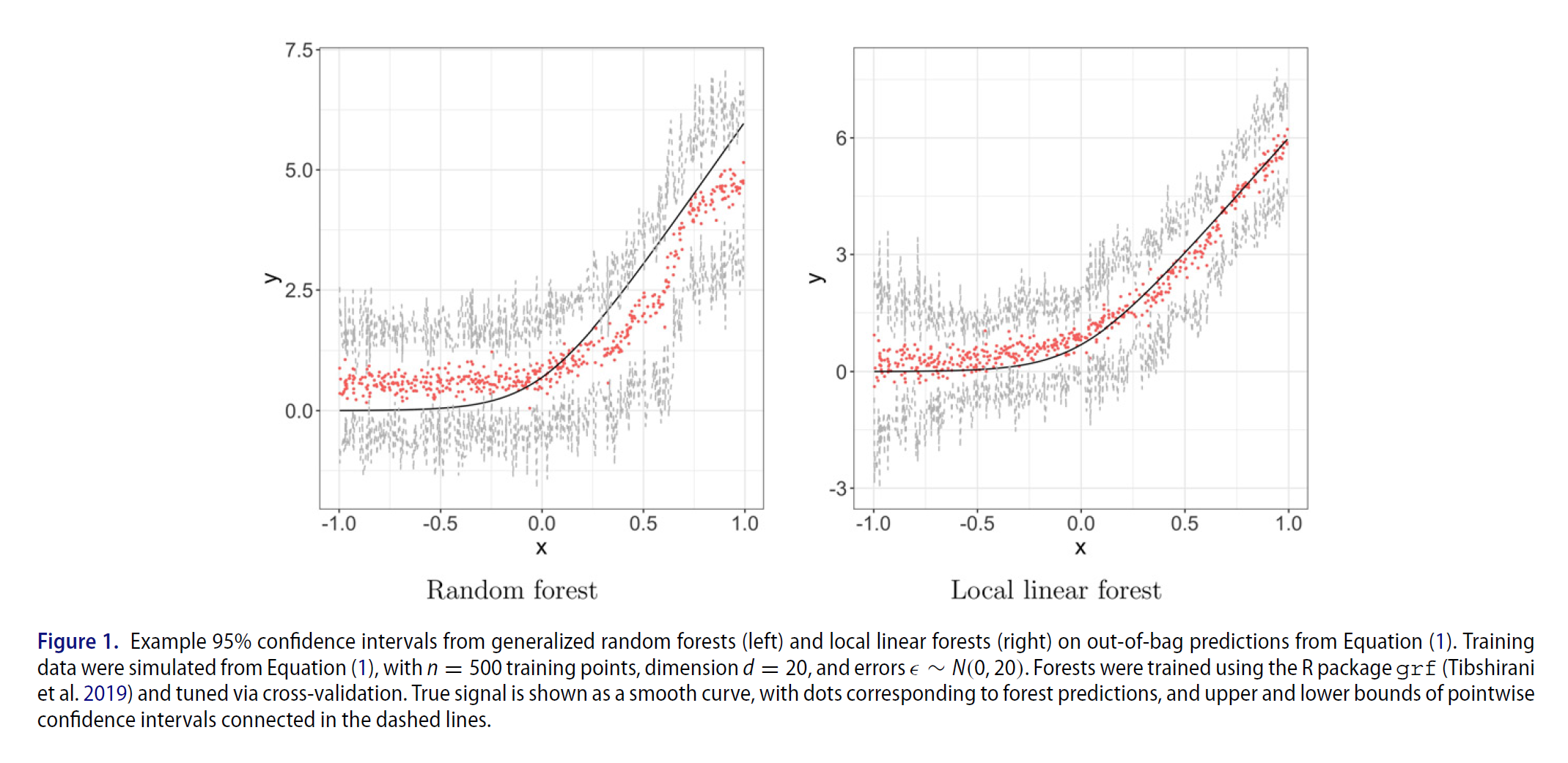
The replication code:


library(randomForest)
library(grf) 
citation("grf")
TT <- 500 # Obervations
P <- 20 # covariates
X <- lapply(rep(TT, P), runif, min=-1, max= 1) 
X <- do.call(cbind, X)
eps <- lapply(rep(TT, 1), rnorm)
eps <- do.call(cbind, eps)
Y <- log( 1 + exp(6*X[,1]) ) + eps # response
rf0 <- randomForest(x= X, y= Y) # standard RF
llf0 <- ll_regression_forest(X= X, Y= Y) # local linear forest
p_llf0 <- predict(llf0) # fitted values