Few weeks back I simulated a model and made the point that in practice, the difference between Bayesian and Frequentist is not large. Here I apply the code to some real data; a model for Industrial Production (IP).
Explanatory variables are only Unemployment Rate (UR) and the Short Rate (SR), interaction between the two and non-linear effect in the form of squared regressors. All variables are in first differences. Will be interesting to see what is the difference in inference this time around, when we do not know the real value of the coefficients.
A natural start is the simple regression:
|
1 2 3 4 5 6 7 8 9 10 11 12 13 14 15 16 17 18 19 20 21 22 23 24 25 26 27 28 29 30 31 32 33 |
dat = as.matrix(read.table(file = "https://dl.dropbox.com/u/9409065/UnemployementData.txt") ) par(mfrow = c(3,1)) plot(dat[,1], ty = "l", main = "Unemployment Rate", xlab = "Time (1960 - 2012, Monthly)", ylab = " ") plot(dat[,2], ty = "l", main = "Short Rate", xlab = "Time (1960 - 2012, Monthly)", ylab = " ") plot(dat[,3], ty = "l", main = "Industrial Production",xlab = "Time (1960 - 2012, Monthly)", ylab = " ") IP <- diff(dat[,3]) UR <- diff(dat[,1]) SR <- diff(dat[,2])) n <- length(IP) nam <- c('Const','Unemployment Rate','Short Rate', 'Interaction', 'Squared Unemployment Rate', 'Squared Short Rate') X <- cbind(rep(1,n),UR,SR, UR*SR, UR^2, SR^2) colnames(X) <- nam simple_regression <- lm(IP~0+X) summary(simple_regression) # Coefficients: # Estimate Std. Error t value Pr(>|t|) # XConst 0.1502 0.0193 7.78 3.1e-14 *** # XUnemployment Rate -0.9028 0.0988 -9.14 < 2e-16 *** # XShort Rate 0.1039 0.0446 2.33 0.020 * # XInteraction -0.0265 0.1857 -0.14 0.887 # XSquared Unemployment Rate -0.7906 0.2972 -2.66 0.008 ** # XSquared Short Rate -0.0140 0.0217 -0.64 0.521 # --- # Signif. codes: 0 ‘***’ 0.001 ‘**’ 0.01 ‘*’ 0.05 ‘.’ 0.1 ‘ ’ 1 # # Residual standard error: 0.419 on 621 degrees of freedom # Multiple R-squared: 0.244, Adjusted R-squared: 0.237 # F-statistic: 33.5 on 6 and 621 DF, p-value: <2e-16 |
As expected, both UR and SR are important (though endogeneity may be at play here), interaction does not add and seems that there is also a non-linear effect of UR.
Now we run the Bayesian regression and the Bootstrap, using same functions from the previous post.
|
1 2 3 4 5 6 7 8 9 10 11 12 13 14 15 16 17 18 19 20 21 22 23 24 25 26 |
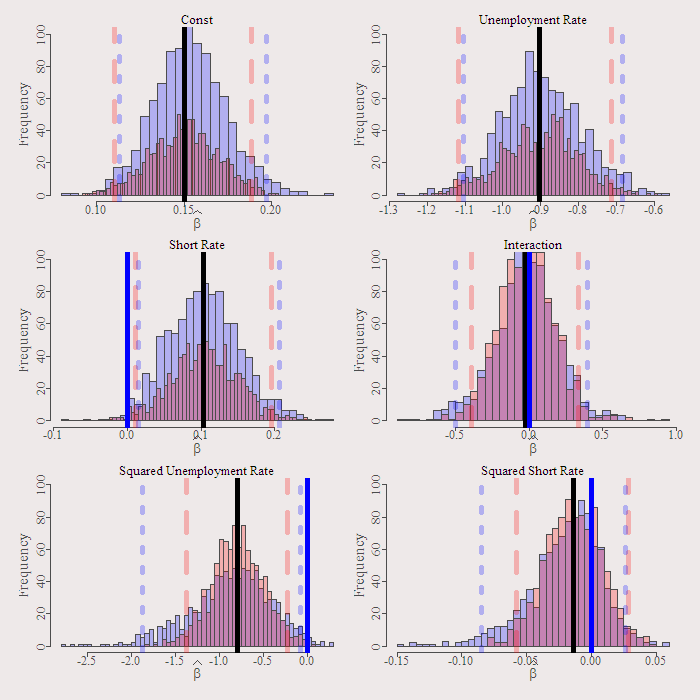
Bmod <- Bayes_reg(dependent=IP, regressors=X) Fmod <- bootbet(dependent=IP, regressors=X) ###plots col1 <- rgb(0,0,1,1/4) col2 <- rgb(1,0,0,1/4) lwd1 <- 5 par( mar=c(3.5,3.3,1.9,1.1)) plotfun0 <- function(l){ hist(Fmod[,l],breaks = 44, col=col1, add=F, ylim = c(0,100), xlab = expression(widehat(beta)) ,main = nam[l] ) hist(Bmod$b_hat[,l], breaks = 44, col=col2, add=T) abline(v=Bmod$lin_mod$coef[l], col = 1, lwd = lwd1) abline(v=quantile(Bmod$b_hat[,l],.975), lty = 2, col = col1, lwd = lwd1) abline(v=quantile(Bmod$b_hat[,l],.025), lty = 2, col = col1, lwd = lwd1) abline(v=quantile(Fmod[,l],.975), lty = 3, col = col2, lwd = lwd1) abline(v=quantile(Fmod[,l],.025), lty = 3, col = col2, lwd = lwd1) abline(v=0, lty = 1, col ='blue', lwd = lwd1) } par(mfrow = c(3,2)) for (i in 1:6){ plotfun0(i) } |
We get the following figure:

As you can see, implementation of both is easy. When the Bayesian and the Frequentist agree you gain better conviction, my intuition is that they agree more often than not.
Some more (good) light reading: [asa onelinertpl]1439803544[/asa]
Figures of the series can be found here.


