Robust beta

In financial context, $\beta$ is suppose to reflect the relation between a stock and the general market. A broad based index such as the S&P 500 is often taken as proxy for the general market. The $\beta$ , without getting into too much detail, is estimated using the regression:

$stock_i = \beta_0+\beta_1market_i+e_i$

A $\widehat{\beta_1}$ of say, 1.5 means that when the market goes up 1% the specific stock goes up 1.5%. (Ignoring all the biases at the moment!)

The way the $\beta_1$ is estimated is using the least squares method, which minimizes the squared distances between the observed value and the fitted value, i.e. $\sum_1^Te_i^2$ . An alternative is to minimize, not the squared distance but the absolute distance, i.e. $\sum_1^T\mid e_i \mid$ . Unlike the least squares, this technique has no closed form solution. Nevertheless, it is easy to find the solution using numerical methods. Most statistical software has already built in the procedure under the name robust regression, or quintile regression. The reason for the name robust regression is that an outlier do not weigh more as it moves further from the fitted line, same way the median of the sequence {1,2,3} is still the same as the median of the sequence {1,2,27}, unlike the mean. So the second procedure is robust to any such values that do not reflect the day to day relationship. The reason for the name quintile regression is that the solution just happens to fit, not the mean, given the explanatory, but the median, given the explanatory, the median is the 50% quintile, hence quintile regression.

Illustration:

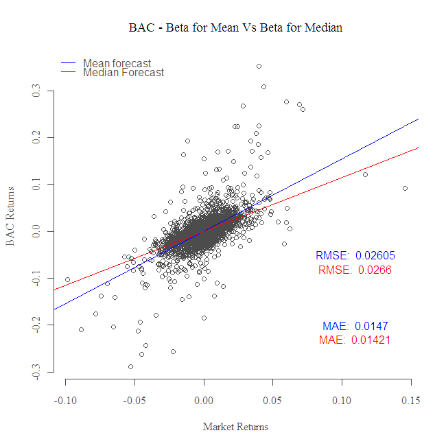
I use returns of “Bank of America” (BAC) as the individual stock, the SPY ETF (Exchange Traded Fund) as a proxy for market returns. Time span is from 1998-09-18 till 2011-09-18, so 13 years of daily data. Let us have a look at the two methods, the least squares and the quintile regression. The former take care of the squared residuals, the latter, the absolute residuals.

: Rubost Regression VS. OLS

What you can see is that the blue line, that correspond with the OLS, or the mean regression, is tilted in the direction of the outliers. The red line on the other hand, is more robust, it does not care about the value of the observations, only about their relative location, and so its slope is more moderate. The robust $\widehat{ \beta}$ is 1.15 while the OLS $\widehat{\beta}$ is 1.54. You can see that the RMSE = Root Mean Squared Error for the blue line is smaller, for the red line the MAE = Mean Absolute Error is smaller.Each method cares about its own metric.

So what is the $\beta$ of Bank of America? My tendency is towards the robust version, I understand that the tails are part of the distribution, but by definition, most days are not outliers. More often than not, truth might be found somewhere in the middle..


end= format(Sys.Date(),"%Y-%m-%d") 
start= format(as.Date("1998-09-18"),"%Y-%m-%d")
library(quantmod)
library(magrittr)
dat0 = getSymbols("BAC", src="yahoo", from=start, to=end, auto.assign = FALSE) %>% as.matrix
dat1 = getSymbols("SPY", src="yahoo", from=start, to=end, auto.assign = FALSE) %>% as.matrix
NROW(dat0)== NROW(dat1) # check if both tickers contain all days
n <- NROW(dat0)
ret = (dat0[2:n, 4]/dat0[1:(n-1),4] - 1) # BAC returns
ret_spy = (dat1[2:n, 4]/dat1[1:(n-1),4] - 1) # SPY retuns
bet = lm(ret~ret_spy)$coef[2] # OLS beta
library(quantreg)
rbet = rq(ret~ret_spy)$coef[2] # Robust beta
plot(ret~ret_spy, main = "BAC - Beta for Mean Vs Beta for Median", xlab = "Market Returns",	ylab = "BAC Returns")
abline(lm(ret~ret_spy)$coef[1:2], col = 4)
abline(rq(ret~ret_spy)$coef[1:2], col = 2)
legend("topleft", bty = "n", c("Mean forecast", "Median Forecast"), col = c(4,2), lty = c(1,1))
text(.11,-.05, paste("RMSE: ",format(sqrt(mean((lm(ret~ret_spy,)$fit - ret^2)),digits = 4)), col = 4)
text(.11,-.08, paste("RMSE: ",format(sqrt(mean((rq(ret~ret_spy,)$fit - ret)^2)), digits = 4)), col = 2)
text(.11,-.2, paste("MAE: ",format(mean(abs(lm(ret~ret_spy,)$fit - ret)), digits = 4)), col = 4)
text(.11,-.23, paste("MAE: ",format(mean(abs(rq(ret~ret_spy,)$fit - ret)), digits = 4)), col = 2)