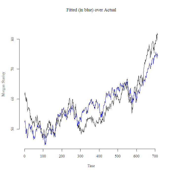
Spurious Regression Illustrated

Spurious Regression problem dates back to Yule (1926): “Why Do We Sometimes Get Nonsense Correlations between Time-series?”. Lets see what is the problem, and how can we fix it. I am using Morgan Stanley (MS) symbol for illustration, pre-crisis time span.  Take a look at the following figure, generated from the regression of MS on the S&P, actual prices of the stock, actual prices of the S&P, when we use actual prices we term it regression in levels, as in price levels, as oppose to log transformed or returns.

The results from the regression are:

	Estimate	Std. Error	t.value	P.value
(Intercept)	-46.4234	2.1827	-21.27	0.0000
beta.hat	0.8534	0.0178	47.90	0.0000
R^2 = 0.76

The graph looks fine, and the results make sense, but utterly wrong!

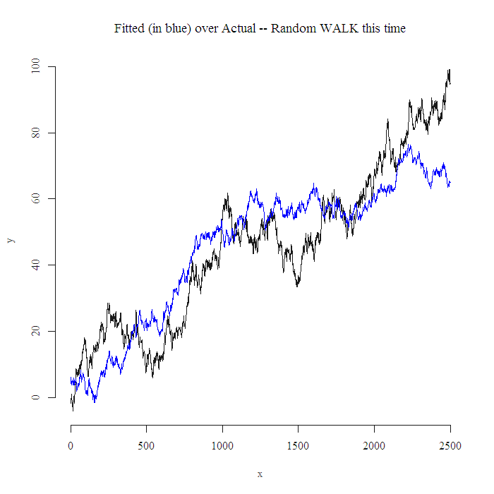
Thing is, the two series are upward drifting, so.. they drift together, it seems as if they are related. As a matter of fact, they are related, but what we just did is the wrong way to check it. Here is similar results from x and y random walks!!

	Estimate	Std.Error	t.value	P.value
(Intercept)	7.0474	0.4651	15.15	0.0000
x	0.5862	0.0062	94.29	0.0000
R^2 = 0.78

Note the resemblance with the previous figure and table.
So.., analysis of two Random Walks which are clearly independent from each other by construction, and the analysis of two time series in levels can have same qualitative result, as if there is a significant positive correlation, that can’t be good right?
In real life, how would I know if what I see is an actual relation or the result of two unrelated series that, just so happen, are drifting in the same direction.

Here we step into the domain of the highly important yet amazingly boring of Unit Roots. This post is not about unit roots, and I want to keep it short not to lose the remaining 5% out of the 100% who started reading. Being abusive, it is suffice to say we need to remove the drift in the series, check here and reference therein for more information.
Once the drift is removed, we can verify that indeed there is a real relation, meaning Morgan Stanley stock movement is actually affected by the market movement. Removing the drift is easy, use returns or first differences. Feel important by telling your classmates that the series are not stationary, hence the transformation.

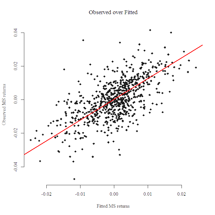
We can transform the data from levels to returns and re-execute the regression as follows:

Now we can see that even after analyzing using returns, not levels, we still get a good fit.

You can use the “adf.test” function in package “tseries” to check if your series drift (stationary*) or not.

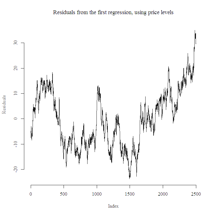
As a final note, fact that we cannot make any inference using price levels does not render the regression completely useless. Both “MS” and “S&P” series are NOT stationary, but together they ARE co-integrated, which is the main justification behind pairs trading. Co-integrated means that y-series may drift, x-series may drift, but the residual from the regression will not!

See how the residuals from the regression fluctuate around zero.

Comments
1. * — stationary process does not only mean “no drift”, we have weak definition and strong definition, see here for more information.
2. according to the graph it seems that it was a good time to short MS and hedge with the market at the end end of the time span I used, which is start of 2007. I leave it to the reader to check what would have been the loss on such a trade.

Some Excellent Readings
Regression Modeling Strategies
Financial Econometrics: From Basics to Advanced Modeling Techniques
A Companion to Theoretical Econometrics
Financial Econometrics: Problems, Models, and Methods
Time Series Analysis