Shrinkage in statistics

Shrinkage in statistics has increased in popularity over the decades. Now statistical shrinkage is commonplace, explicitly or implicitly.

But when is it that we need to make use of shrinkage? At least partly it depends on signal-to-noise ratio.

Introduction

The term shrinkage, I think, is the most underappreciated umbrella term in statistics. The reason is that it is often masked under different names. Take the widely used RiskMetrics estimator for volatility:

$\sigma^2_{t+1} = \lambda \sigma^2_{t} + (1-\lambda) r_{t}^2.$

What do we see here? if $E(r_t) = 0$ (assuming for example that expected return for the day is zero), the $r_{t}^2$ term is simply an estimate for the volatility based only on today’s observation. With $\lambda= 0.94$ (chosen arbitrarily) we simply exert strong pull over the volatility estimate which is based only on the one observation, pushing it towards that estimate which is based on the full sample so far: $\sigma^2_{t}$ . This heavy pull (0.94-heavy) is a shrinkage towards a “grand total”. You are now a step further to recognize shrinkage whichever way you look. Bayesian methods and forecast ensembles to name only a couple of topics. It is all shrinkage.

One shrink and one no-shrink

On Thursday, February 9th 2017, one of the strongest statistical minds passed away. James Stein shocked the statistical world when in 1961 he showed that the Maximum Likelihood Estimation (MLE) method which we love so much, can be bested using but a pinch of shrinkage. The amazement was complete when it was shown that dominance is uniform (as oppose to case-specific, or for a particular region of the parameters).

Thinking regression, I admit the intuition is absent. “Let me tell you what you should do: use unconstrained excellent optimizer” (OLS) “once you are done, you better bias it.” You would think that if the results would be better by biasing, the optimizer would deliver the better version directly and already. The reason why this is not the case is very nuanced and is related to Optimism of the Training Error Rate.

Let’s skip the formulae for the James Stein (JS) shrinkage estimator and go directly to the code. In a simulated regression settings, we can compute the MLE (which is also the OLS) and then see what is the shrinkage we need to apply based on the JS estimator. Simulating 100 observations with 10 explanatory variables, each of which has a coefficient of one.


TT <- 100 # 100 observation
p <- 10 # 10 explanatories
X <- matrix(nrow = TT, ncol = p)
X <- apply(X, 2, rnorm)
sdd <- 10
eps <- rnorm(TT, mean=0, sd= sdd)
bet <- rep(1,p)  # the real unknown coefficients
y <- t(t(bet)%*%t(X) + eps)
dat <- data.frame(y= y, X)
mle <- lm(y~ X - 1, data= dat) # MLE, regression without intercept
round(summary(mle)$coef[,1], 1) # the resulting MLE estimates
beta_mle <- mle$coef 
mu_mle <- t(beta_mle %*% t(X)) # the expectation given the estimates
# Let's get the James–Stein estimator
sig <- summary(mle)$sigma
xprimex <- t(X)%*%X
B <- 1 - ( (p-2)* (sig^2) ) / ( t(beta_mle) %*% xprimex %*% beta_mle )
print(B)
    [,1]
[1,] 0.78

TT <- 100 # 100 observation

p <- 10 # 10 explanatories

X <- matrix(nrow = TT, ncol = p)

X <- apply(X, 2, rnorm)

sdd <- 10

eps <- rnorm(TT, mean=0, sd= sdd)

bet <- rep(1,p) # the real unknown coefficients

y <- t(t(bet)%*%t(X) + eps)

dat <- data.frame(y= y, X)

mle <- lm(y~ X - 1, data= dat) # MLE, regression without intercept

round(summary(mle)$coef[,1], 1) # the resulting MLE estimates

beta_mle <- mle$coef

mu_mle <- t(beta_mle %*% t(X)) # the expectation given the estimates

# Let's get the James–Stein estimator

sig <- summary(mle)$sigma

xprimex <- t(X)%*%X

B <- 1 - ( (p-2)* (sig^2) ) / ( t(beta_mle) %*% xprimex %*% beta_mle )

print(B)

[,1]

[1,] 0.78

Ok, we need to take our MLE estimate for beta and shrink it by 0.78:


> cat(beta_mle)
-0.329 1.59 1.63 1.62 3.13 0.0172 1.09 3.3 1.91 2.14
> beta_js <- B * beta_mle
> cat(beta_js)
-0.256 1.24 1.27 1.26 2.44 0.0134 0.847 2.57 1.49 1.67

> cat(beta_mle)

-0.329 1.59 1.63 1.62 3.13 0.0172 1.09 3.3 1.91 2.14

> beta_js <- B * beta_mle

> cat(beta_js)

-0.256 1.24 1.27 1.26 2.44 0.0134 0.847 2.57 1.49 1.67

You can see that the coefficient are now pulled towards zero, which is why they call it shrinkage.

Of course, the in sample RMSE is better using the MLE:


mu_mle <- t(beta_mle %*% t(X))
mu_js <- t(beta_js %*% t(X))
ev = function(actual,prediction){
rmse= sqrt(mean((actual-prediction)^2)) 
}
ev(y, mu_mle)
[1] 9.01
ev(y, mu_js)
[1] 11.2

mu_mle <- t(beta_mle %*% t(X))

mu_js <- t(beta_js %*% t(X))

ev = function(actual,prediction){

rmse= sqrt(mean((actual-prediction)^2))

}

ev(y, mu_mle)

[1] 9.01

ev(y, mu_js)

[1] 11.2

But, going forward? Let’s simulate from the same setting new data 500 times (500 different possible futures say) and use our estimates obtained from before, going forward:


RR <- 500
rmse_mle <- rmse_js <- NULL # make accuracy containers
for (i in 1:RR){
newX <- matrix(nrow = TT, ncol = p) # generate new X
newX <- apply(newX, 2, rnorm) # generate new X
eps <- rnorm(TT, mean=0, sd= sdd) # generate new Y
newy <- t(t(bet)%*%t(newX) + eps) # generate new Y using same parameters
new_mu_mle <- t(beta_mle%*%t(newX)) # new y.hat MLE 
new_mu_js <- t(beta_js %*% t(newX)) # new y.hat JS 
rmse_mle[i] <- ev(newy, new_mu_mle) # Accuracy MLE
rmse_js[i] <- ev(newy, new_mu_js) # Accuracy JS
}

RR <- 500

rmse_mle <- rmse_js <- NULL # make accuracy containers

for (i in 1:RR){

newX <- matrix(nrow = TT, ncol = p) # generate new X

newX <- apply(newX, 2, rnorm) # generate new X

eps <- rnorm(TT, mean=0, sd= sdd) # generate new Y

newy <- t(t(bet)%*%t(newX) + eps) # generate new Y using same parameters

new_mu_mle <- t(beta_mle%*%t(newX)) # new y.hat MLE

new_mu_js <- t(beta_js %*% t(newX)) # new y.hat JS

rmse_mle[i] <- ev(newy, new_mu_mle) # Accuracy MLE

rmse_js[i] <- ev(newy, new_mu_js) # Accuracy JS

}

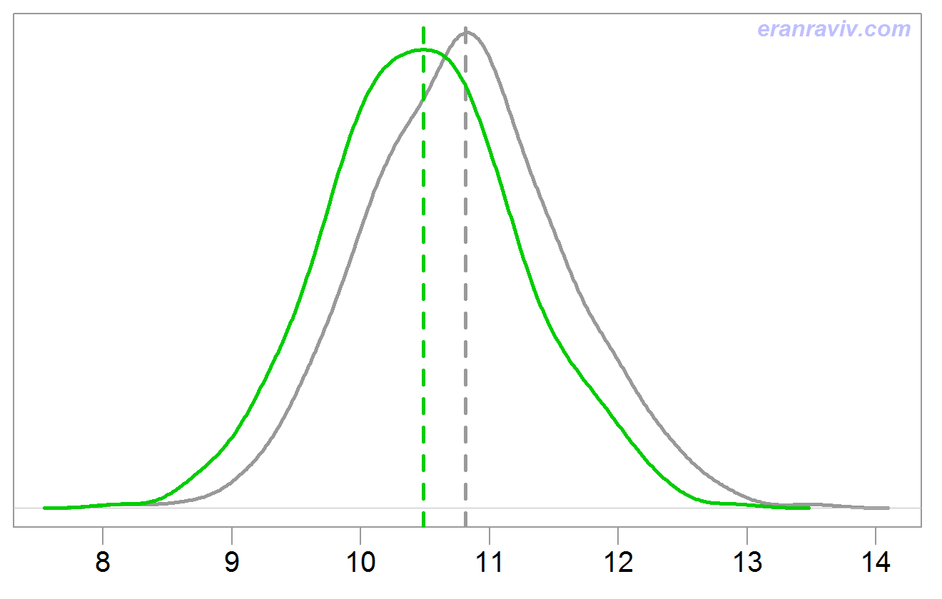
Plotting the results we see that the James Stein Estimator is more accurate than the MLE estimate.

We don’t always need shrinkage. You may have noticed the sdd argument in the first code-chunk above. We have set it to 10. The bet was set to 1. This means that the signal is quite weak compared with the noise, which is exactly when we would like to shrink. Changing sdd to 1, and executing the same code again delivers the following vanilla figure:

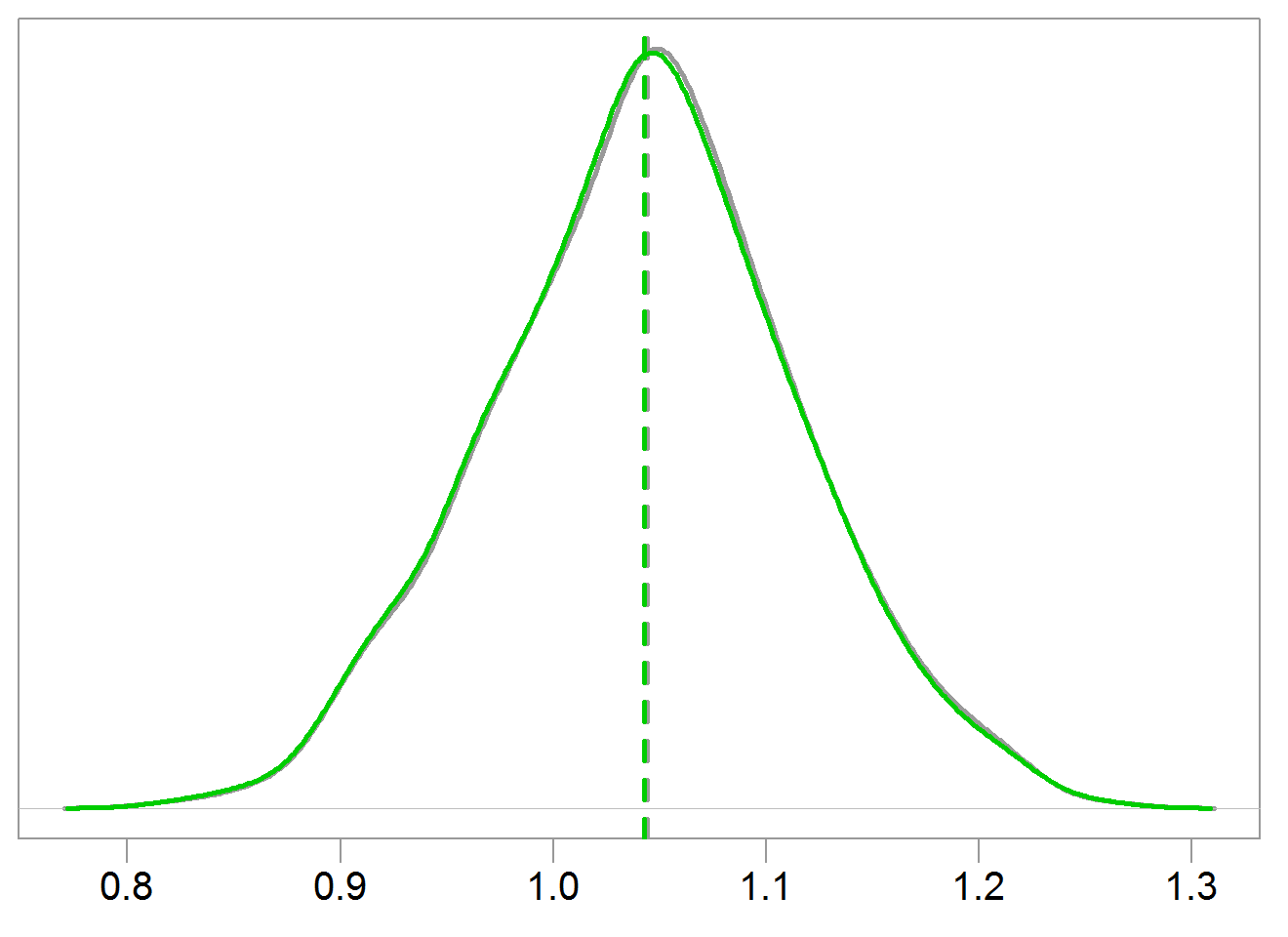
If the signal-to-noise ratio is reasonable, we don’t need to call shrinkage techniques to our aid.

What about the theory underpinning statistical shrinkage? Thus far, despite great efforts there is no proper analogy for the optimality theory found in unbiased estimation literature. There is no theory to help us choose the correct amount of shrinkage we should apply. We know shrinkage can be advantageous, but almost that is it. Therefore, data-driven method such as cross-validation are now standard, despite computational difficulties and the lack of theoretical assurance (after all, theoretical assurance is just that).

Very recently, from econometrics rather than statistics, a paper titled: “Efficient shrinkage in parametric models” by Prof. Hansen echos the 1961 Stein’s paper in that “if the shrinkage dimension exceeds two, the asymptotic risk of the shrinkage estimator is strictly less than that of the maximum likelihood estimator (MLE).” The ‘parametric models’ in the title means the paper is concerned with shrinkage applied to estimates which were obtained using MLE. In the paper there is a derivation which seems to me analogous to the term B in our code above. But in a more general setting (equations 10-13 in the paper). A must-read for those interested in shrinkage estimation (free download below).

After you’ve read this, you may wonder how the MLE method survives those brutal attacks. Why keep using MLE if there is more accurate estimators out there? There are good reasons, but we discuss this in another post.