Moving average is one of the most commonly used smoothing method, basically the go-to. It helps us detect trend in the data by smoothing out short term fluctuations. The computation is trivial: take the most recent k points and simple-average them. Here is how it looks:
Moving average example with k= 24 (simulated data)
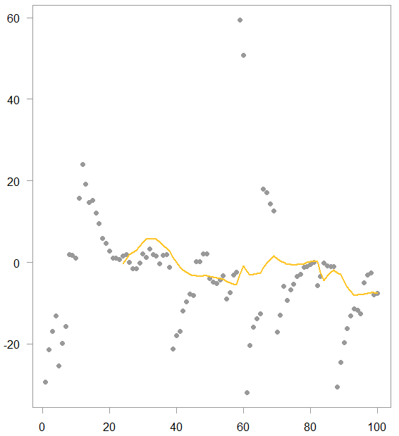
As you can see we have a few points which are stretched out. Those data points pull the moving average towards their values. They do so until they exit the averaging window.
Another look at the moving average
Looking from a different angle, the moving average can also be thought of as a solution of a linear regression with only an intercept. How so? say you have 24 points ( ) without any explanatory variables. The average is the
  value, the intercept, which minimizes the sum of squared residuals in a regression of the form
  (check if you want).
Now that we have cast the moving average computation in a regression settings, the door is open to use all the fine regression tooling at our disposal. Specifically, we don’t have to use a squared residuals loss function  in that regression. We can retrieve the intercept by minimizing other loss functions. Boom.
For example, why should an equities boom or doom periods pull the (estimated) trend as quickly as they do? Put differently, your preference may be to wait a bit until you are better convinced the tables have turned. This means that you need a bit of tweaking to tailor your moving average to fit your needs, i.e. risk profile. On offer, here are couple of ways you can do that. I rely heavily on a post I wrote not too long ago (Adaptive Huber Regression).
Using robust loss functions to robustify your moving average
We can use two different loss functions, the one is the least absolute deviation, the other is the Huber loss function. Let’s simulate some data and plot it to see how the moving average (ma from here on) differ in each case.
<pre class="lang:r minimize:false decode:true" title=" The Distribution of the Sample Maximum as a function of the number of observations">
library(magrittr)
library(quantreg)
library(MASS)
# citation("MASS")
# citation("quantreg")
# citation("magrittr")

TT <- 100
x= arima.sim(model=list(ar = c(0.8)), n=TT, rand.gen = rt, df=1) %>% as.numeric
wind= 24
# r for robust
# h for huber
rma <- hma <- maa <- NULL
for (i in 1:(TT - wind+1)){
maa[(i+wind-1)] <- lm(x[i:(i+wind-1)] ~ 1)$coef
hma[(i+wind-1)] <- rlm(y= x[i:(i+wind-1)], x= rep(1, wind), maxit = 200)$coef
rma[(i+wind-1)] <- rq(x[i:(i+wind-1)] ~ 1)$coef
}
And this is how it looks like:
Moving average example with k= 24 (simulated data), for different loss functions
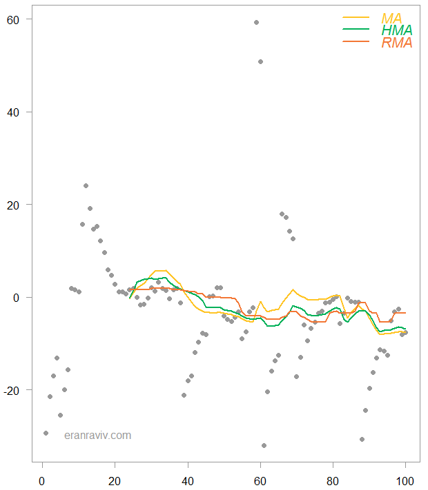
The yellow line is the same as before. The green line is from the Huber loss function and the red line is for a least absolute deviation loss function. As you can see, you need more than just a handful of observation to get the HMA (huber moving average) excited. The RMA (robust moving average) which is basically a moving median is the least variable of the three.
If you read this you are well familiar with the EMA (exponential moving average). Here we are basically advocating the reverse. These alternative MA specifications outlined here can be of use when you are looking for ways to stabilize\dampen the impact of few singular observations, so you can collect proof for until you are convinced you see an actual turn, for example.


