Beauty.. really? well, beauty is in the eye of the beholder.
One of the most striking features of using Maximum Likelihood (ML) method is that by merely applying the method, conveniently provides you with the asymptotic distribution of the estimators. It can’t get more general than that. The “how you do”, not the “what you do” permits proper inference. The only caveat, though indeed a considerable one, is that the data generating process:
![\[(1) \qquad f(y \vert x, \theta_0)\]](https://eranraviv.com/wp-content/ql-cache/quicklatex.com-9d29f44b307d4a37f81d6500a8287bf2_l3.svg "Rendered by QuickLaTeX.com")
needs to be correctly specified. As an aside we see from the simple formula that the ML is really conditional (on X) ML. If your guess for the density of  is correct, there isn’t much more to be desired. The ML method delivers consistent, low variability estimate and impressively, its distribution. However, what happens if your guess for the density is not correct? meaning you, as we all do, misspecify the model.
As it turns out, the estimates are not consistent anymore. Funny enough, the shape of the distribution of the estimates are similar, just the center is different (Huber 1967). Not to be disheartened just yet (as I am sure you are..), Quasi-Maximum Likelihood (QML) to the rescue.
The term “Quasi” here means “to a certain extent” or “almost”. We can still use the ML method and hope that the model is incorrect specifically, but correct more generally. There are special cases in which despite the fact that we have a bad guess for the density in (1) we can still recover good estimates. By far the most frequently used likelihood is (conditional) normal, but say the variable follows a different conditional distribution. How different? say it is a Poisson process. You can go right ahead with your normal specification. In fact, if the density belongs to the so-called ‘linear exponential family’ (LEF) it should be fine. Other distributions included in the LEF are binomial and exponential. So even if you have the wrong specification but you are still in within the “family” your estimates are still consistent, remarkably.
- Illustration
Simulate  from the model
  where once
  and once
  . One set of simulation has 50 observations only (small sample) and another set has 1000 observations (large sample), so as to give a feel for the harm of misspecifiying the density. In both cases we apply ML using maximum likelihood which is normal. Here are the results:
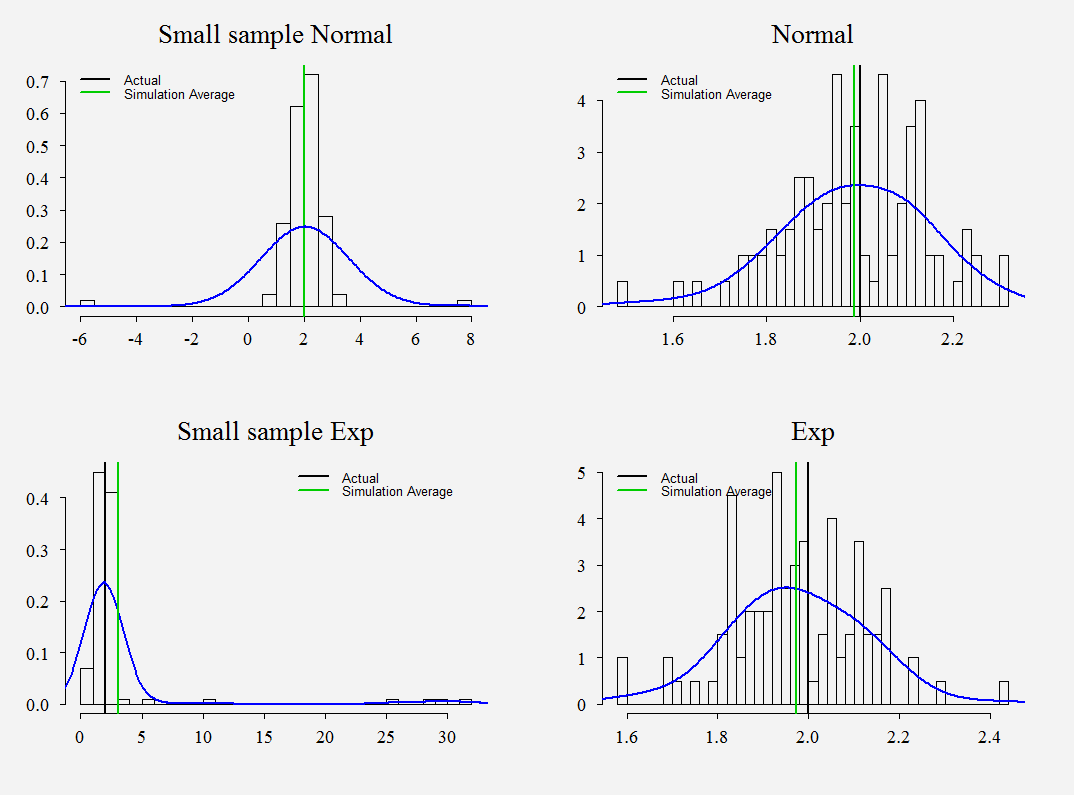
Those are histograms of  , we have 100 simulations. The vertical black is the arbitrary number of 2 chosen as the unknown value. The green is the average of the 100 simulations. Trivially, we see that it is better to have a good guess for the density. When the sample is small, the estimate from the misspecified model are awful, the correctly specified model has its ‘glitches’, but nothing dramatic compared with the misspecified one. However, add more data and.. voila.
Lastly, if we use normal likelihood in both cases; when our guess for the density is right but also when it is wrong (I mean in reality we don’t know if it’s right or not), how do we know when to call what we do ML and when to call it “almost” ML? Essentially, calling your estimation method QML allows you to humbly admit you are not sure about the density, but you hope it is within the LEF so that you preserve consistency of the estimates.
Good readings


The code
# The likelihood function
lik <- function(par,X,Y) {
p <- dim(X)[2]
xbeta <- X%*%par[1:p]
Sig <- par[(p+1)]
-sum(-(1/2)*log(2*pi)-(1/2)*log(Sig^2)-(1/(2*Sig^2))*(Y-xbeta)^2)
}
# Simulate from the model above
TTs <- 50; TT <- 500; p=1
RR <- 100
rpar <- c(1,2)# intercept=1, slope=2; arbitrary choice
parametersE <- parametersN <- parametersNs <- parametersEs <- matrix(nrow=RR,ncol=p+2)
for (i in 1:RR){
x <- runif(TT) # Simulate variable
x <- cbind(rep(1,TT),x) # Add intercept
p <- NCOL(x) # correct p
xs <- x[1:TTs,] # create small x data
epsnorm <- rnorm(TT) # normal noise
epsexp <- rexp(TT) # funny looking noise
ynorm <- x%*%rpar + epsnorm # create y
yexp <- x%*%rpar + epsexp # create y
ynorms <- ynorm[1:TTs] # create small y
yexps <- yexp[1:TTs] # create small y
noisepar <- c(c(rpar,1)+rnorm((p+1),0,0.5)) # create different starting values
MLE <- optim(par=noisepar,lik, Y=ynorm,X=x,method = "CG")
MLEs <- optim(par=noisepar,lik, Y=ynorms,X=xs,method = "CG")
parametersN[i,] <- MLE![par parametersNs[i,] <- MLEs](https://eranraviv.com/wp-content/ql-cache/quicklatex.com-c327585142e7d82b8f7b5eb7ffc8d2b4_l3.svg "Rendered by QuickLaTeX.com") par
MLE <- optim(par=noisepar, lik, Y=yexp, X=x, method="CG")
MLEs <- optim(par=noisepar, lik, Y=yexps, X=xs, method="CG")
parametersE[i,] <- MLE
par
MLE <- optim(par=noisepar, lik, Y=yexp, X=x, method="CG")
MLEs <- optim(par=noisepar, lik, Y=yexps, X=xs, method="CG")
parametersE[i,] <- MLE![par parametersEs[i,] <- MLEs](https://eranraviv.com/wp-content/ql-cache/quicklatex.com-058fc33c438bf308ad5274c170abd6b1_l3.svg "Rendered by QuickLaTeX.com") par
}
# figure
par(mfrow=c(2,2))
mbw <- 0.3
mbws <- mbw*20
hist(parametersNs[,2],freq = F,main="Small sample Normal",xlab="",ylab="",breaks=44)
abline(v=2,lwd=2)
legend("topleft", c("Actual", "Simulation Average"),lwd=2,col=c(1,3),bty="n")
abline(v=mean(parametersNs[,2]),lwd=2,col=3)
lines(density(parametersNs[,2],width = mbws),col=4,lwd=2)
hist(parametersN[,2],freq = F,main="Normal",xlab="",ylab="",breaks=44)
abline(v=2,lwd=2);lines(density(parametersN[,2],width = mbw),col=4,lwd=2)
abline(v=mean(parametersN[,2]),lwd=2,col=3)
legend("topleft", c("Actual", "Simulation Average"),lwd=2,col=c(1,3),bty="n")
hist(parametersEs[,2],freq = F,main="Small sample Exp",xlab="",ylab="",breaks=44)
abline(v=2,lwd=2);lines(density(parametersEs[,2],width = mbws),col=4,lwd=2)
abline(v=mean(parametersEs[,2]),lwd=2,col=3)
legend("topright", c("Actual", "Simulation Average"),lwd=2,col=c(1,3),bty="n")
hist(parametersE[,2],freq = F,main="Exp",xlab="",ylab="",breaks=44)
abline(v=2,lwd=2);lines(density(parametersE[,2],width = mbw),col=4,lwd=2)
abline(v=mean(parametersE[,2]),lwd=2,col=3)
legend("topleft", c("Actual", "Simulation Average"),lwd=2,col=c(1,3),bty="n")
par
}
# figure
par(mfrow=c(2,2))
mbw <- 0.3
mbws <- mbw*20
hist(parametersNs[,2],freq = F,main="Small sample Normal",xlab="",ylab="",breaks=44)
abline(v=2,lwd=2)
legend("topleft", c("Actual", "Simulation Average"),lwd=2,col=c(1,3),bty="n")
abline(v=mean(parametersNs[,2]),lwd=2,col=3)
lines(density(parametersNs[,2],width = mbws),col=4,lwd=2)
hist(parametersN[,2],freq = F,main="Normal",xlab="",ylab="",breaks=44)
abline(v=2,lwd=2);lines(density(parametersN[,2],width = mbw),col=4,lwd=2)
abline(v=mean(parametersN[,2]),lwd=2,col=3)
legend("topleft", c("Actual", "Simulation Average"),lwd=2,col=c(1,3),bty="n")
hist(parametersEs[,2],freq = F,main="Small sample Exp",xlab="",ylab="",breaks=44)
abline(v=2,lwd=2);lines(density(parametersEs[,2],width = mbws),col=4,lwd=2)
abline(v=mean(parametersEs[,2]),lwd=2,col=3)
legend("topright", c("Actual", "Simulation Average"),lwd=2,col=c(1,3),bty="n")
hist(parametersE[,2],freq = F,main="Exp",xlab="",ylab="",breaks=44)
abline(v=2,lwd=2);lines(density(parametersE[,2],width = mbw),col=4,lwd=2)
abline(v=mean(parametersE[,2]),lwd=2,col=3)
legend("topleft", c("Actual", "Simulation Average"),lwd=2,col=c(1,3),bty="n")


