Density estimation is now a trivial one-liner script in all modern software. What is not so easy is to become comfortable with the result, how well is is my density estimated? we rarely know. One reason is the lack of ground-truth. Density estimation falls under unsupervised learning, we don’t actually observe the actual underlying truth. Another reason is that the theory around density estimation is seldom useful for the particular case you have at hand, which means that trial-and-error is a requisite.
Standard kernel density estimation is by far the most popular way for density estimation. However, it is biased around the edges of the support. In this post I show what does this bias imply, and while not the only way, a simple way to correct for this bias. Practically, you could present density curves which makes sense, rather than apologizing (as I often did) for your estimate making less sense around the edges of the chart; that is, when you use a standard software implementation.
For a start, see for yourself. Assume you would like to estimate the density of the daily market volatility; say estimated by the squared daily return of the SPY, code at the end of the post.
I removed few outliers from the chart for better readability. This is how it looks like if you simply use the default density function in R. The green line is without changing the default bandwidth, while the light blue line is with a more narrow bandwidth.
Distribution of daily market variance, estimated as squared daily return of the SPY ETF. Without boundary correction.
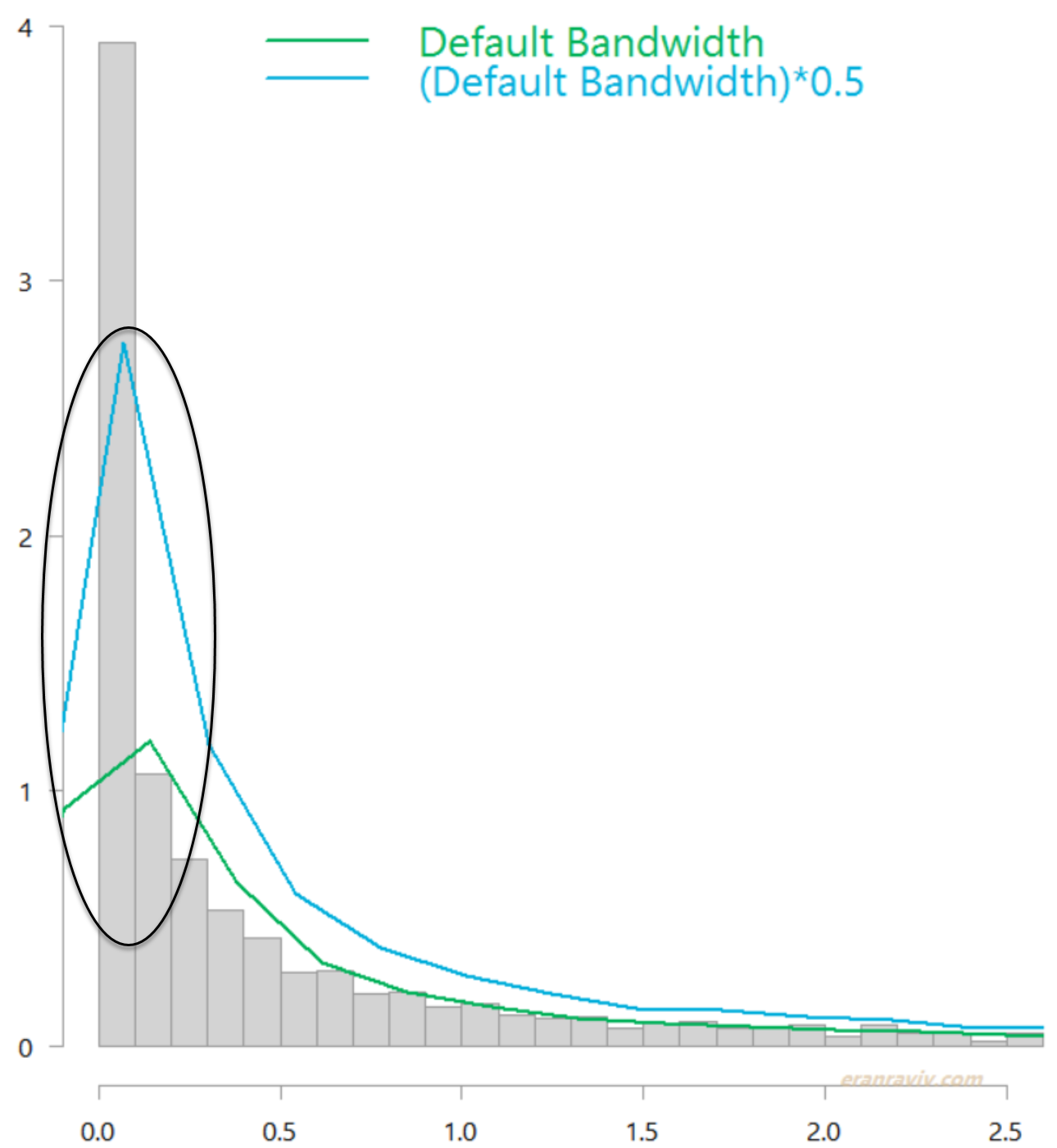
Both are quite ugly estimates in that circled region. You can see that the kernel estimate uses a sort of “moving window”, which falls off the left edge. You would expect the highest density to be just above zero. That is where most of the observations are concentrated (observations are dense there). The “moving window” should not “continue” below zero, as the variance never goes negative and yet it does. This is an example for the bias I was referring to. Jones (1996) offers a simple solution which is conveniently coded for us in the evmix package. Applying it provides the following, much more reasonable estimates:
Distribution of daily market variance, estimated as squared daily return of the SPY ETF. With boundary correction.
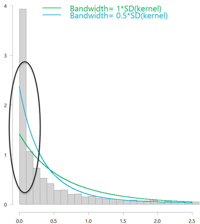
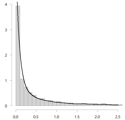
Both those estimate are boundary-bias-corrected, but the window-size (the bandwidth) is a bit off. You can use the bw.nrd function to help choose the bandwidth. It is meant for Gaussian kernels but in my opinion the kernel type is inconsequential here. Using that function, you then get the following figure:
See below for good references and the code.
References
All of Nonparametric Statistics. Currently amazon reviews are averaged 3.5. But given that no one gave it 3 stars, you can imagine people love it or hate it. I myself like it. Professor Larry Wasserman is a world-class statistician. He used to have a very influential blog which he Seinfeldly retired (at it’s pick) at the end of 2013. Unfortunately for all of us lovers of statistics, he has wonderful insights and impressive clarity of exposition.
Jones, M. C., and P. J. Foster. “A simple nonnegative boundary correction method for kernel density estimation.” Statistica Sinica (1996): 1005-1013. Not an easy read without some prior knowledge.
Code
Data and standard kernel density estimation:
|
1 2 3 4 5 6 7 8 9 10 11 12 13 14 15 16 17 18 19 20 21 22 23 24 25 26 |
# The following must be installed # Before this code could be executed smoothly library(quantmod) library(magrittr) library(evmix) citationevmix) k <- 10 # how many years back? end <- format(Sys.Date(),"%Y-%m-%d") start <-format(Sys.Date() - (k*365),"%Y-%m-%d") symetf = c('SPY') dat0 = getSymbols( symetf, src = "yahoo", from= start, to= end, auto.assign = F, warnings = FALSE, symbol.lookup = F ) w1 <- (100*dailyReturn(dat0)) %>% as.numeric %>% "^"(2) w1 %>% head # plot(w1) hist(w1, breaks=1000, xlim= c(0,2.5), freq= F, ylab="", main="", col= "lightgrey") TT <- NROW(w1) tmpp <- w1 %>% density() lines(tmpp, lwd=2) tmpp <- w1 %>% density(adjust = 0.5) # half the BW lines(tmpp, lwd=2) |
Boundary corrected kernel density estimate:
|
1 2 3 4 5 6 7 8 |
# ? dbckden # for help on the function seqq <- seq(0, 2.5, length.out=TT) bc_dens <- dbckden(x= seqq, kerncentres=w1, bw=1) lines(bc_dens~seqq, col=e_col[4], lwd=2) bc_dens <- dbckden(x= seqq, kerncentres=w1, bw=0.3) lines(bc_dens~seqq, col=e_col[4], lwd=2) |


Thanks for sharing the insights. Though I am perhaps too picky to wish that the illustrative example used would have been less “perfect” or more representative of realistic cases one would come across in practice. As it stands, the estimated density looks too close to like simply connecting the height of each histogram bar, not giving a sense of how magical the bw.nrd function could actually be in more realistic cases.