Forecasting the Eurozone Misery index

Is Miss Stagflation coming to visit?
The Misery index is the sum of inflation and unemployment rate. We would like them both to stay naturally low, and we are miserable when they are not. The index is currently floating in it’s record scratching levels. In this post I demonstrate the use of the nice FitAR package in R to fit an AR model and see what we can expect accordingly. Inflation and unemployment numbers concerning the Eurozone (17 countries) can be found here.
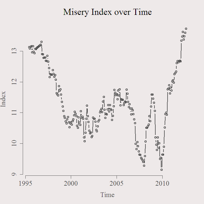
Have a look at the index over time:

An autoregressive model seems to be a reasonable idea and the FitAR package in R is quite flexible so lets use that one. Among the many options you can specify, you can select which lags are more influential according to some criterion. Our data is of monthly frequency so a maximum lag of 12 is a reasonable choice. Once we specify the maximum number of lags we can search for the best subset, according for example to AIC or BIC. The obvious advantage of such a model is its flexibility. We don’t need to model all 12 lags if, say, lag numbers 2 and 4 are not important. In that case, they will be omitted in the selection stage. On the downside, we lose the interpretation, go figure what is the meaning of a selection process which ends up with lags number 4,5 and 10.

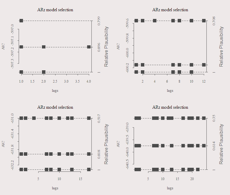
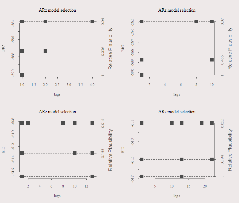
A nice feature of the FitAR package is that the function SelectModel selects the lags in a smart way (according to some algorithm). So we do not scan all possibilities which will take forever, see reference below. The next two figures outline the number of variables and lag order chosen for the two most common criteria, BIC and AIC. There are four graphs corresponding with the maximum number of lags allowed, 6,12,18,24. The three different results correspond with the best three lag structures. You can see how much more likely is the best selection relative to its first runner-up on the right axis, this provides some confident when the difference is large. The left axis is just the value of the criterion, lower is better.

We can see that the BIC criterion is much more restrictive. We can see lag number one is important, as well as lag number two, though to a lesser extent according to Mr. BIC.

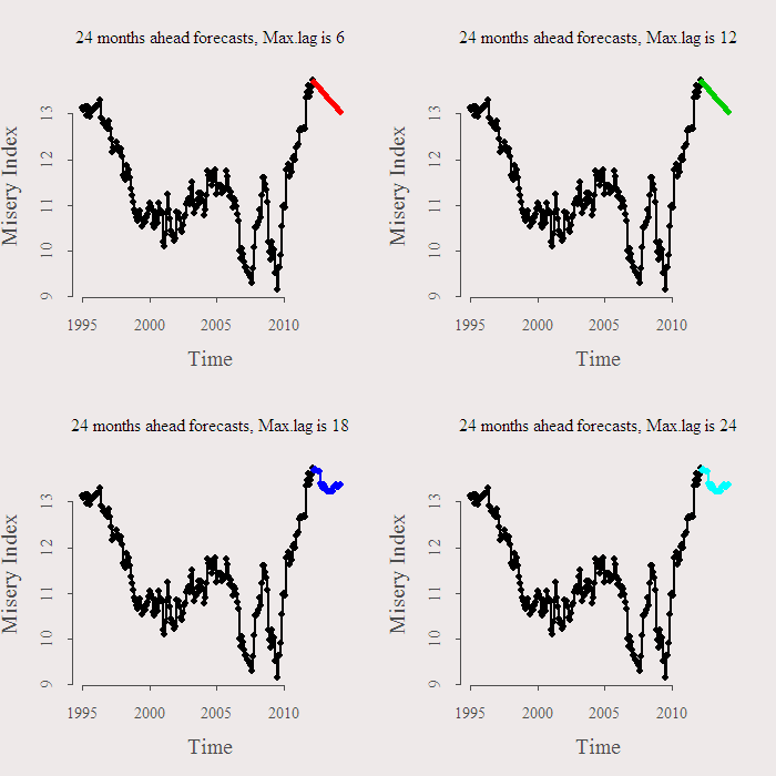
Next is to see what these models tell us about the future. The following figure present the forecast for the next 24 months (BIC only):

The short memory models in the upper half predict that things will get better. However, the “grownup” models, which have longer memory and can tell you something about life, predict that Miss Stagflation is here to stay. Time will tell, I might have a look at the index in the future to see how these forecasts fare. Code and references are below. Thanks for reading.

Notes:
1. ARz means I used standard OLS for the lag structure selection. ARp will give you an ARIMA style which makes interpretation even harder.
2. there is also a good movie called Misery.
Code:

Resources:
PARTIAL AUTOCORRELATION PARAMETERIZATION FOR SUBSET AUTOREGRESSION
[asa onelinertpl]0470272848[/asa]