Contents
Preview
Constructing a portfolio means allocating your money between few chosen assets. The simplest thing you can do is evenly split your money between few chosen assets. Simple as it is, good research shows it is just fine, and even better than other more sophisticated methods (for example Optimal Versus Naive Diversification: How Inefficient is the 1/N). However, there is also good research that declares the opposite (for example Large Dynamic Covariance Matrices) so go figure.
Anyway, this post shows a few of the most common to build a portfolio. We will discuss portfolios which are optimized for:
- Equal Risk Contribution
- Global Minimum Variance
- Minimum Tail-Dependence
- Most Diversified
- Equal weights
We will optimize based on half the sample and see out-of-sample results in the second half. Simply speaking, how those portfolios have performed.
Portfolio-construction, few options
Before we go to the data, first a quick review of the portfolio-construction options at our disposal:
- Equal Risk Contribution
- Global Minimum Variance
- Minimum Tail-Dependence
- Most Diversified
This means that each asset would contribute the same degree of volatility to the portfolio. So if the volatility of asset A is 3x, and the volatility of asset B is 1x, then we need to hold three parts of asset B for every part of asset A (here for exposition purposes we assume that only A and B exist and zero correlation between them).
Still reading? you know this one. Moving on.
I already wrote about tail-dependence in the context of correlation structure and in the context of Extreme Value Theory. I paste from the R help page of the Minimum Tail-Dependence function :
“Akin to the optimisation of a global minimum-variance portfolio, the minimum tail dependent portfolio is determined by replacing the variance-covariance matrix with the matrix of the lower tail dependence coefficients”.
So instead of targeting portfolio’s volatility as the thing to minimize, we input another matrix, the matrix of tail dependence (diagonal is “dismissed” as 1). This matrix is much more noisy to estimate than the covariance\correlation matrix (which is already quite noisy mind you). The reason is explained in the previous correlation structure post.
Using a tail-dependence matrix can dictate much different portfolio than that of the global minimum, due to the correlation structure I spoke about before.
First time for me to hear about this actually. Learning new things is one of the leading drivers for blogging you see. And also why a “quick short post” in my mind turns out to be as lengthy as this one. Indeed, sharing those random thoughts with you doesn’t help brevity, but we are friends so it’s ok.
Look at this ratio:  . In words, it is a weighted average of the individual volatilities divided by the volatility of the portfolio. The nominator is at least as large as the denominator, so the minimum of this ratio is 1, and it is achieved if you have only a single asset.
If you have say two assets which are independent of each other and have the same volatility then the ratio is quickly computed as:
![\[\frac{.5 \sigma + .5 \sigma}{ \sqrt{ .5^2\sigma^2 + .5^2\sigma^2} } = \frac{\sigma}{\sqrt {.5} \sigma }= \frac{1}{\sqrt {.5} } = \sqrt {2},\]](https://eranraviv.com/wp-content/ql-cache/quicklatex.com-b89da5bd6874be321382af6dc04ab360_l3.svg "Rendered by QuickLaTeX.com")
and this can be generalized to N assets. You want this ratio to be as large as possible, which would mean that your portfolio has much lower volatility compared with the individual constituents. See here for a good Most Diversified portfolio reference.
Before we continue just bear in mind that the term diversification is not an exact term or a formal one. When we write correlation we can recall the formula for (linear) correlation between two variables. But the definition of diversification is context-dependent, so the above represents a particular definition in this specific context. Another word other than diversification could easily be chosen.
Package Frapo in R
The large number of portfolio optimization packages can be overwhelming. Just google “Portfolio Construction with R” and see what comes. Enter Bernhard Pfaff. I met him during the 2016’s R in Finance excellent conference where he gave a talk about portfolio selection with multiple criteria objectives. He is the maintainer of the FRAPO package which I will be using in this tutorial. The FRAPO package is efficient (read: C++ engine) and friendly, as you will see from the very few lines of code below.
We start by pulling data on the three tickers: 'SPY','TLT', 'IEF'. Those are ETF’s servicing us as proxies for stocks (US) long term bonds (US) and short term bonds (US) respectively. We will use weekly returns and split the data in halves. The first half is used for portfolio optimization, and the second half is used to examine how those portfolio have performed. No rebalancing, no slippage or trading costs incorporated.
|
1 2 3 4 5 6 7 8 9 10 11 12 13 14 15 16 17 18 19 20 21 22 23 24 25 26 27 |
library(quantmod) k <- 10 # how many years back? end<- format(Sys.Date(),"%Y-%m-%d") start<-format(Sys.Date() - (k*365), "%Y-%m-%d") symetf = c('SPY','TLT', 'IEF') l <- length(symetf) w0 <- NULL for (i in 1:l){ dat0 = getSymbols(symetf[i], src="yahoo", from=start, to=end, auto.assign = F, warnings = FALSE, symbol.lookup = F) w1 <- weeklyReturn(dat0) w0 <- cbind(w0,w1) } time <- as.Date(substr(index(w0),1,10)) w0 <- as.matrix(w0) colnames(w0) <- symetf # head(w0) # Let's split the sample in two parts # Create a portfolio based on first part and # See how it is doing in the second part t_insample <- NROW(w0)/2 tmpind <- 1:t_insample w0_insample <- w0[tmpind, ] w0_outsample <- w0[-tmpind, ] |
Now and build them following portfolios using the code below:
|
1 2 3 4 5 6 7 8 |
library('FRAPO') # install if not yet, using install.packages citation("FRAPO") ERC <- PERC(Sigma= cov(w0_insample) )@weights # Equal Risk Contribution GB <- PGMV(Returns= w0_insample)@weights # Global Minimum Variance MTD <- PMTD(Returns= w0_insample)@weights # Minimum Tail-Dependence MD <- PMD(Returns= w0_insample)@weights # Most Diversified |
And those are the resulting portfolio weights:
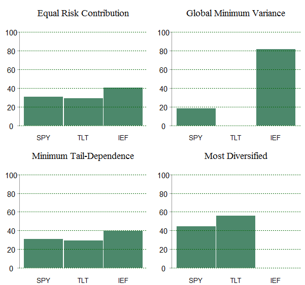
In the chart above we can see that:
Global Minimum Variance needs short term bonds (IEF) the most. Equal Risk Contribution does not have much larger weight compared with the other two which is somewhat surprising. Most Diversified takes the “two ends”; Stock and Bonds, while IEF which is more like cash is left out. Finally Minimum Tail-Dependence looks a bit like the Equal Risk Contribution, which tells me that the tail dependence (as estimated here) is not very different than the volatility. Or perhaps more accurately, the relative considerations don’t change when we input tail-dependence matrix instead of the correlation matrix).
Now lets see how those portfolios performed on the second half of our sample.
Distribution of daily returns per year
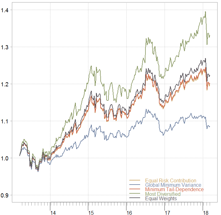
Looks like Equal Risk Contribution, Minimum Tail-Dependence and Equal weights are not very far apart. Most Diversified and Global Minimum Variance differ. The latter has only lukewarm performance while the Most Diversified is doing very well. On the whole, the main driver of results here is how much money you hold in the IEF ETF (which is close to cash in a way). The more short term bond you have (IEF), the less return you make. Of course, the Global Minimum Variance is doing exactly what is supposed to be doing. That is, looking at the recent downturn it has the smallest draw-down.
Finally, we can compute the mean over the variance of returns (not annualized, just on weekly frequency).
Distribution of daily returns per year
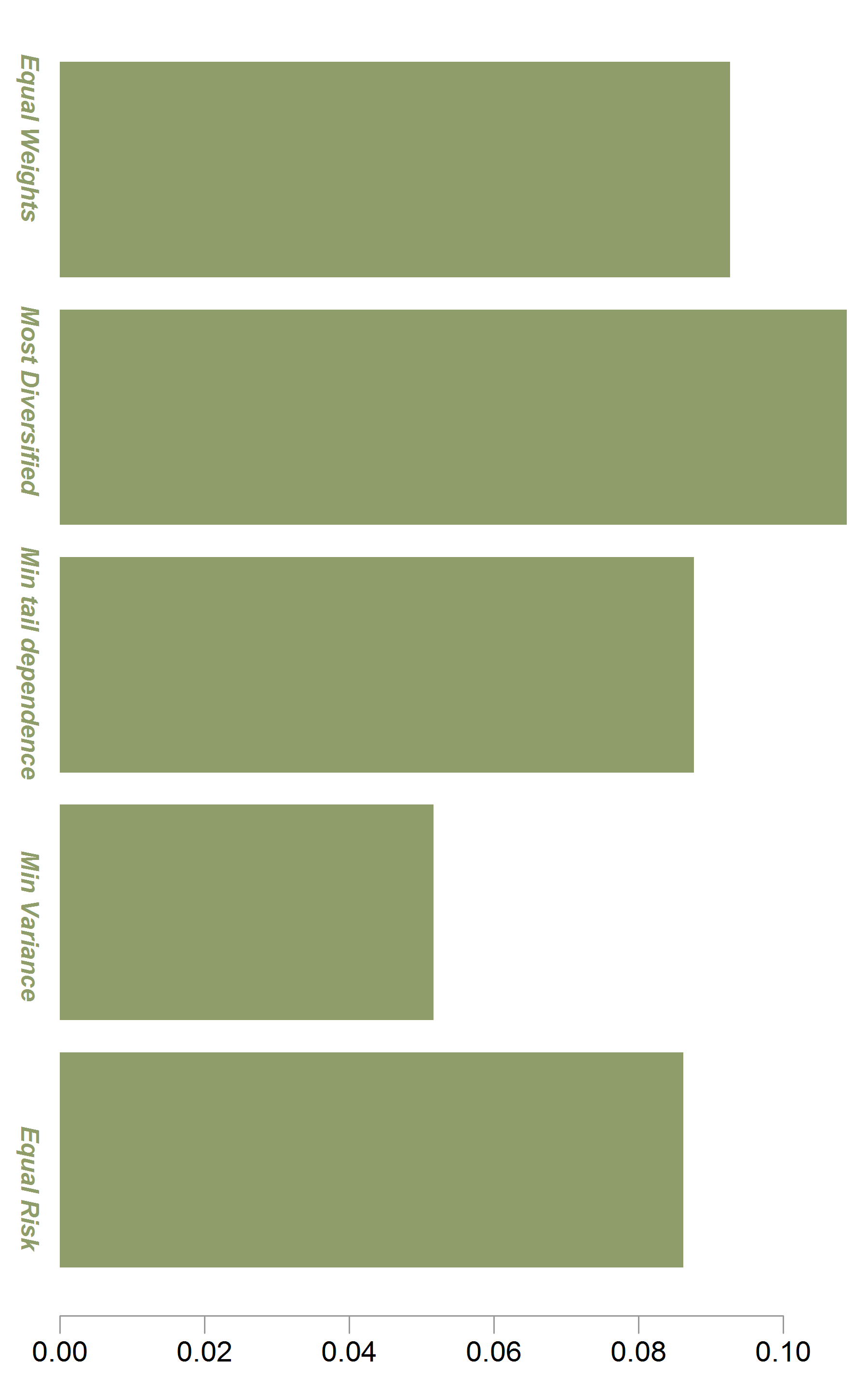
Apart from the Global Minimum Variance, I would say you simply get paid for the volatility you are willing to endure. At least looking at weekly returns, there is not an awesome difference between the portfolios.
What will happen if we use say 100 other US equity tickers? I suspect the differences are even less pronounced. So it only matters when you are talking big money, or maybe if you have less correlation between the different portfolio components, I think.
If you enjoyed this post and you like those kind of comparisons have a look at this book: Global Asset Allocation: A Survey of the World’s Top Asset Allocation Strategies You can buy it by paying roughly the price of a double espresso, or you can simply register here and get a kindle version after a few days (by doing this you agree to review the book).
Appendix
Some requested code
|
1 2 3 4 5 6 7 8 9 10 11 |
tmp_tab <- cbind(ERC, GB, MTD, MD) colnames(tmp_tab) <- c("Equal Risk Contribution", "Global Minimum Variance", "Minimum Tail-Dependence", "Most Diversified") ports <- w0_outsample %*% cbind(tmp_tab/100, 1/l) cum_ret <- matrix(nrow= NROW(ports), ncol= NCOL(ports) ) for(j in 1:NCOL(ports)) { for( i in 1: NROW(ports) ) { cum_ret[i, j] <- prod( (1+ports[1:i,j]) ) - 1 } } 52*(ports %>% apply(2, mean)) |


Thanks for this great analysis. Very informative…would you please mind sharing the rest of the code on the out of sample covering the charts?
Regards,
Updated.
If you had a “like” button I would have hit that instead of commenting. I particularly enjoyed the work you din on the various types of volatility some years back (Parkinson, Garman-Klass etc, though my fav is Yang-Zhang but you did not talk about that). Good stuff, please keep it up. Frank
Good to hear. You are very welcome.
Thank you for the great example. Would you please share the code for plotting the performance graphs and barplots for weights.
Sir,
It has been like an amazing resource for practice for me, as in my MSc , we only study theory and hardly any practical are there. One thing in regards to portfolio i wished to know like if we want to combine all these portfolios into one mother portfolio like a mutual fund, but then how we assign the weights for them and do benchmarking.
Thank you for the kind words. As to your question, check here. You can also create simulation, where you yourself dictate what are the optimal individual weights and assign each portfolio construction method the optimal weights based on performance.
Could you maybe share the code for the plot of how the portfolios performed on the second half of the sample? Thanks in advantage!
Dear Dr. Eran Raviv,
Thank you for your blog and sharing. I hope you are doing fine in this pandemic.
If you dont mind, I would like to have one request. I read the book of Dr. Bernhad, I could not find rebalancing code either.
I tried many times but I still fail. So, is it possible that you provide rebalancing code under FRAPO (the above example?), please?
Thank you so much