What is tail dependence really? Say the market had a red day and saw a drawdown which belongs with the 5% worst days (from now on simply call it a drawdown):
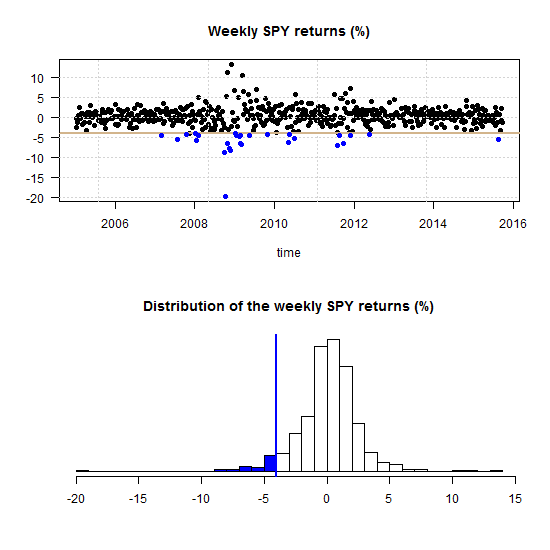
One can ask what is now, given that the market is in the blue region, the probability of a a drawdown in a specific stock?
We all understand the concept of beta of a stock with respect to the market, the sensitivity of a stock with respect to market (for example the S&P 500). The concept of tail dependence is similar in that it is the sensitivity of a stock to a drawdown in the market. If each time the market drops, the stock drops it would mean two things:
1. The probability of a drawdown in a stock is 100%, given the market already dropped.
2. The stock is very sensitive to market drawdowns
It is intuitive to think that such a measure would go hand in hand with high beta. But it is not one to one. It can very well be that a stock with high beta could be less sensitive to a drawdown compared to another stock with low beta.
Formally, the dependence in the left tail of a stock to the left tail of the market is defined as:
(1) 
where Q is some quantile which depends on how you define what is a tail, in our example 5%. From probability, if two events are independent, the probability of seeing both events is the multiplication of the probability of each:
(2) 
where A here is the event:  , and B is the event
  . Empirically what we do for estimation is simply to count the number of points that lie below the 5% cutoff of the stock, for each of the points that lie below the 5% region of the market. This function use this concept to measure the tail dependence between two time series:
# The cc parameter defines the tail. Default to 5%
corstruc <- function(seriesa, seriesb, cc = 0.05){
# stop if the two series are not in the same length
if(length(seriesa)!=length(seriesb)){stop("length(seriesa)!=length(seriesb)")}
TT <- length(seriesa)
# make container
condcor=NULL
# count how many are lower than 5%
ind0 <- ifelse(seriesa<quantile(na.omit(seriesa),cc),1,0)
ind <- which(ind0==1)
# given that series a is lower than 5% (meaning had a drawdown) count how many in series b
ind1 <- sum(ifelse(seriesb[ind]<quantile(na.omit(seriesb),cc),1,0))
# compute the probability
pr0 <- ind1/TT # probability that both dropped
return(list(PR = pr0))
}
Let us pull ten ETFs and have a look how different is the beta from the tail dependence measure. We pull the tickers and transform to weekly returns.
 library(quantmod)
sym = c('XLY','XLP','XLE','XLF','XLV','XLI','XLB','XLK','XLU','SPY')
l=length(sym)
end<- format(Sys.Date(),"%Y-%m-%d")  ; start<-format(as.Date("2005-01-01"),"%Y-%m-%d")
dat0 = (getSymbols(sym[1], src= "yahoo", from=start, to=end, auto.assign = F))
n = NROW(dat0)
w0 <- NULL
for (i in 1:l){
dat0 = getSymbols(sym[i], src="yahoo", from=start, to=end, auto.assign = F)
w1 <- weeklyReturn(dat0)
w0 <- cbind(w0,w1)
}
time <- index(w0)
ret0 <- 100*as.matrix(w0) # more to percentage points
colnames(ret0) <- sym
Now we compute the beta and the tail dependence measure, and plot it.
 pr <- bet <- NULL
for(i in 1:(l-1)){
	bet[i] <- lm(ret0[,l]~ret0[,i])$coef[2]
	pr[i] <- corstruc(ret0[,l], ret0[,i])
	}
barplot(bet, names.arg  = sym[-l], col = "lightblue", las = 1)
title(main   = "Beta with respect to the S&P 500")
barplot(unlist(pr), names.arg  = sym[-l], col = "lightblue", las = 1)
abline(h = 0.05^2, col = 3, lwd = 4)
title(main = "Tail dependence with the S&P 500")
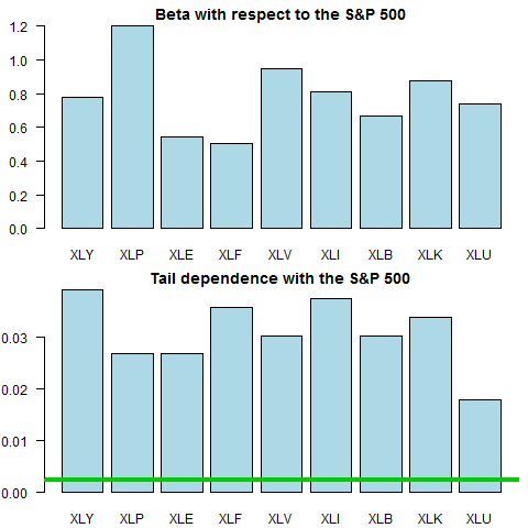
The green line is  which is what we should expect from two completely (tail) independent series.
I recently read the short and nice paper from the oven of the Dutch National Bank: The simple econometrics of tail dependence (Maarten R.C. van Oordt and Chen Zhou). The word simple in the title refers to the fact that this simple concept above outlined, can be considered using a regression settings. They show that the bottom panel of the second chart can be equally reached at using the interceptless regression:
(3) 
where  is an indicator function for when the event A happens, the stock exhibit a drawdown. Have a look:
five_quan <- quantile(ret0[,l], 0.05)
indl <- ifelse(ret0[,l] < five_quan, 1, 0)
bet_dependence <- NULL
for(i in 1:(l-1)){
	five_quan <- quantile(ret0[,i], 0.05)
	indk <- ifelse(ret0[,i] < five_quan, 1, 0)
	bet_dependence[i] <- lm(indk ~ 0 + indl)$coef[1]
}

Ok, it is the same, so what?
So instead of working with difficult multidimensional copulas and struggle with convergence issues, we can use what we know about regression and extend the analysis to a multivariate case. How likely it is that we see a drawdown in A given not only a drawdown in B, but a drawdown in B, C and D. Their paper demonstrates that extension using U.K., U.S., German and French stock market returns. The paper is short because it was published in Economic Letters, so a few things more to say and perhaps do:
– We can make inference, but not using the usual STD of the regression coefficient since it is an indicator regression (so usual assumptions do not apply). We need to use block bootstrap.
– We have to include interactions as well for inference to be valid.
– An idea which I will not pursue further is to improve estimates using what we know about modern regression; LASSO, BAGGING etc.
As a final word, I was wondering what is up with the XLU (Utilities) ETF, why is it that the tail dependence looks weak relative to the beta, and how is the picture different than for say the XLY (Consumer Discretionary).
plot(ret0[,"XLU"]~ ret0[,"SPY"], main = "XLU~SPY (weekly returns, %)", ylab = "XLU", xlab = "SPY", las = 1)
lines(lowess(ret0[,"XLU"]~ ret0[,"SPY"]), lwd = 2, col = 4)
plot(ret0[,"XLY"]~ ret0[,"SPY"], ylab = "XLY", xlab = "SPY", main = "XLY~SPY (weekly returns, %)", las = 1)
lines(lowess(ret0[,"XLY"]~ ret0[,"SPY"]), lwd = 2, col = 4)
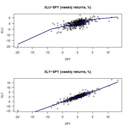
Looks as if our estimates are sensitive to some extreme observations. Perhaps robust regression would deliver more stable estimates, so that is another extension possible. I leave it at that.


Wouldn’t tail dependence for sector ETFs be directly correlated with the sector weights wrt SPY?
In other words a self fulfilling thing, sectors with high weightings would show much of the same characteristics that the index shows.
In short, you are correct. Those estimates are biased in that sense.
As I write in the post itself, in Maarten and Zhou paper they use country stock indexes, so no bias there (at least not due to this specific endogeneity issue).
Very interesting findings.
I would guess Consumer Discretionary would hurt the most when market turns south. Since people would shop less luxury goods, eat out less in those occasions. Utilities would hurt less, since people still need gas, heat, etc.
P(A given B)=P(A intersection B)/P(B) = P(A) in case of independence, so instead of using 0.25%, you should be using 5% as a boundary for independence. But as you noticed, it has to exactly equal to 5% for independence and in case this is not so, technically it is dependent. But as your probability is a function of the sample size, you might want to test for statistical significance of your probability estimate in order to be sure.