Statistical Shrinkage (2)

During 2017 I blogged about Statistical Shrinkage. At the end of that post I mentioned the important role signal-to-noise ratio (SNR) plays when it comes to the need for shrinkage. This post shares some recent related empirical results published in the Journal of Machine Learning Research from the paper Randomization as Regularization. While mainly for tree-based algorithms, the intuition undoubtedly extends to other numerical recipes also.

While bootstrap aggregation (bagging) use all explanatory variables in the creation of the forecast, the random forest (RF from hereon) algorithms choose only subset. E.g. for 9 explanatories you randomly choose 3, and create your forecast using only those 3. In that sense, bagging can be thought of as a degenerate RF where randomization is applied only across rows, but not across columns. It’s therefore natural to compare and quantify the difference between the two – to help disentangle the contribution of randomization applied to rows from that applied to columns.

One of the nice exercises in the paper is to artificially inject noise to some real data, then plot the difference in performance of the RF versus bagging; this as a function of the amount of noise added. Specifically they look at the quantity

$\mathrm{RTE}=\frac{\widehat{\operatorname{Err}}(\mathrm{Bagg})-\widehat{\operatorname{Err}}(\mathrm{RF})}{\hat{\sigma}_y^2} \times 100 \%$

Broadly speaking, it’s the difference between the accuracy achieved by bagging and the accuracy achieved by RF. A positive number means RF is more accurate. Here is what they find on that: 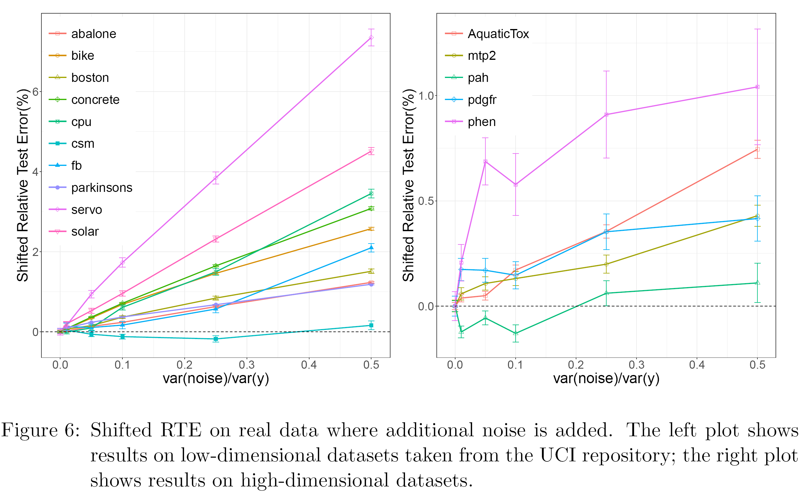Different lines represent different datasets. The X-axis is the amount of injected noise to the data. You see the lines are on average upward sloping. Implying that the lower the signal-to-noise (higher noise) the more accurate RF is, relative to bagging. I wish the right chart would have the same y-axis as the one on the left because it’s a bit misleading as is, but the point is valid: the lower the SNR the larger the benefits from shrinking.

Common practice is to cross-validate your way to a satisfactory shrinking hyperparameter. While this paper does not develop a full-blown theoretical ground to walk on, it does open the door to some well-wished heuristics. Low signal-to-noise calls for more randomization. Indeed, the next thing to do is to be able to estimate the signal-to-noise ratio in our data, and the shrinking parameter should follow.

Why RF is (almost like everything else..) shrinkage?

The acquisitive readers may note that this post uses the terms “shrinkage” and “randomization” interchangeably.

Why so?

Insight is gained from Theorem 2 in the said paper. It states that if we are in a (1) standard regression setup and (2) we have an orthogonal design, where all explanatory variables are independent then the following intuitive result holds

$\hat{\boldsymbol{\beta}}^{\text {ens }} \stackrel{B \rightarrow \infty}{\longrightarrow} \frac{m}{p} \hat{\boldsymbol{\beta}}^{O L S}$

The coefficient for the eventual forecast is the same as the OLS one, times $\frac{m}{p}$ (B for bootstrap samples). So for example say that you choose randomly m=3 explanatory variable out of your existing p=9, then in effect you use the OLS coefficient times 1/3. Or put more clearly, you follow the equation $\frac{3}{9} \times \beta_{ols} + \frac{6}{9} \times 0$ .

Finally, I mentioned that this insight is extended to other domains. The Dropout procedure directly comes to mind. While there are many narratives behind the success of Dropout in deep learning application I bet it’s just, quite simply, shrinkage applied in a high SNR domains.