The mean is arguably the most commonly used measure for central tendency, no no, don’t fall asleep! important point ahead.
We routinely compute the average as an estimate for the mean. All else constant, how much return should we expect the S&P 500 to deliver over some period? the average of past returns is a good answer. The average is the Maximum Likelihood (ML) estimate under Gaussianity. The average is a private case of least square minimization (a regression with no explanatory variables). It is a good answer. BUT:
There is a lot of historical inertia in play. Often times, most of the times I dare say, you can estimate the mean more accurately. The way forward is using robust estimation.
To compute the trimmed mean, aka truncated mean if you fancy, you simply discard observations in the tails of the distribution when computing the average. For example, you trim observations which are above the 90% quantile or below the 10% quantile, computing the average only based on those observations which sitting in between the 90% quantile and the 10% quantile.
Doing this, and if the distribution is symmetric, you will enjoy more accurate estimate for the mean. More accurate in the sense that you will be closer to the actual unknown parameter. The gains are particularly large for heavy tail distribution, hence the relevance. Of course we don’t know beforehand if the distribution is symmetric or not, heavy tailed or not. Although there are many cases where simply applying common sense would do. For example we can safely assume a good degree of symmetrical distribution when discussing hourly, daily, or even weekly equity returns.
If the distribution is not symmetric it does not directly mean that we are at a loss. But the benefits of the trimmed mean are less of a clear cut. There is a bias-variance tradeoff if the distribution is asymmetric.
Illustration
The following code lets you examine those statements made above. You can change the number of simulations, the length of the vector (TT), how much you would like to trim (trimm), how much asymmetry you want to introduce. how heavy you would like the tails to be, and how light you would like the tails to be; for comparison purposes.
trim_mean_example <- function(Simulations= 200, TT= 100, trimm= 0.1, ncpp= 0, df_heavy= 4, df_light= 30) {
	for (i in 1:Simulations){
		xheavy <- rt(TT, df= dfheavy, ncp= ncpp)
		xlight <- rt(TT, df= dflight, ncp= ncpp)
		mtrim_heavy[i] <- mean(xheavy, trim= trimm)
		mtrim_light[i] <- mean(xlight, trim= trimm)
		m_light[i] <- mean(xlight)
		m_heavy[i] <- mean(xheavy)
	}
	return(list(m_light= m_light, mtrim_light= mtrim_light, m_heavy= m_heavy, mtrim_heavy= mtrim_heavy))
}
out <- trim_mean_example()
We can plot the results:
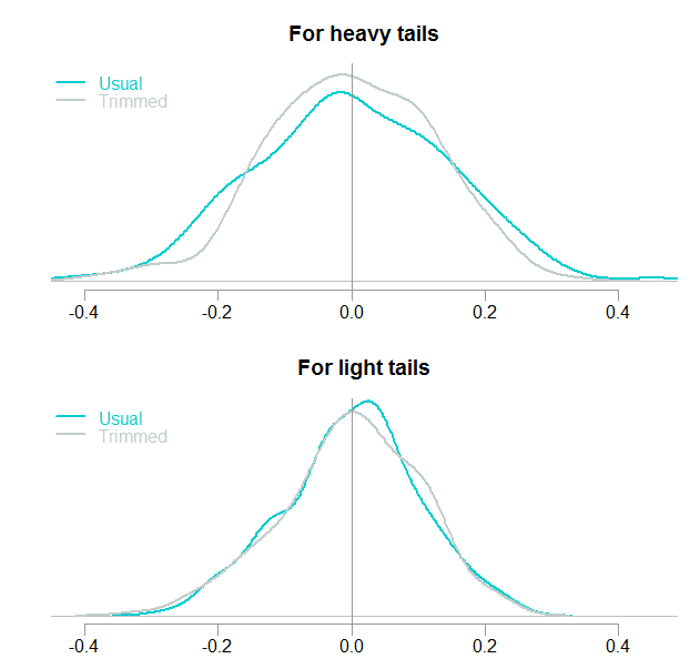
We know the mean is zero in this case since it was simulated as such. You can see the distribution of the simulated estimates. The trimmed version is closer to the actual mean, with less probability of “falling” too far. If the tails are light – in this example it is essentially normal distribution, there is not much gain; but no much loss neither.
Let’s change the non central parameter which is also responsible for the degree of distributional asymmetry. Before it was set to 0, now we set it to 1 and re-run the code,
out <- trim_mean_example(ncpp=1) :
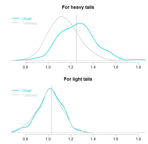 The price we pay for gaining accuracy when the distribution is symmetric is clearly visible. The top panel shows the effect brought about by trimming: a biased estimate. Strong bias when the tails are heavy, not much bias for the light-tail version. The vertical lines represent the theoretical mean, they can be computed using an ugly-looking expression for the mean of a Noncentral t-distribution. The values are 1.25 (top) and 1.03 (bottom). Although the estimate is biased after trimming, it is not entirely clear we bear a negative cost. Downwards bias, sure, but lower variance as well. To compute the ultimate price of using the trimmed mean when the distribution is asymmetric we need a cost function, which we will not get into here. That cost function would determine how unhappy we are to get it wrong in whichever direction.
This is more than a theoretical curiosity
Right or wrong, many are using the average of past returns as a guidance for expected future returns. If you run the following code you will discover the mean estimate of daily US equity return is materially higher using a trimmed mean estimate.
symetf = c('SPY')
end<- format(Sys.Date(),"%Y-%m-%d")
start<-"2000-01-01"
l = length(symetf)
dat0 <- lapply(symetf, getSymbols, src="yahoo", from=start, to=end,
               auto.assign = F, warnings = FALSE, symbol.lookup = F)
xd <- dat0[[1]]
retd <- 100*(as.numeric(xd[2:NROW(xd),4])/as.numeric(xd[1:(NROW(xd)-1),4]) -1)
mean(retd)
mean(retd, trim= 0.1)
Apart from that, there is a lot riding on mean estimation. The X.bar, denoting the usual average as an estimate for the mean is the go-to plug-in estimate in all walks of modern statistics. Replacing the average, with a truncated average as an estimate for the mean is not a free lunch. But, as I mentioned, I think it is underutilized due to historical inertia. Start making the substitution where appropriate- with a robustified version is often better for you than the standard version. Maximum Likelihood estimation is not dying, but it is old.
Some further reading
Fundamentals of Modern Statistical Methods: Substantially Improving Power and Accuracy

Understanding and Applying Basic Statistical Methods Using R


Seems like bad advice to me. Why not just use the median? It also estimates the mean in the symmetric case. Or better yet, use maximum likelihood with an appropriate distribution, and you do not even need to assume symmetry. With trimming (and Winsorizing), it is not clear what you are estimating in general, and it is not clear that the estimand (whatever it is) is a relevant target.