Convolutional Neural Networks (CNNs from here on) triumph in the field of image processing because they are designed to effectively handle strong spatial dependencies. Simply put, adjacent pixel-values are close to each other, often changing only gradually from one pixel to the next. In a picture where you wear a blue shirt, all the pixels in that area of the picture are blue. You can think of a strong autocorrelated time series, just for spatial data rather than sequential data. This post explains few important concepts related to CNNs: sparsity of connections, parameter sharing, and hierarchical feature engineering.
Contents
Convolutional Neural Networks
Googling “CNN” you typically find explanations about the convolution operator which is a defining characteristic of CNN, for example the following animation:
This is quite different from images that you see for general neural networks which are NOT convolutional neural networks:
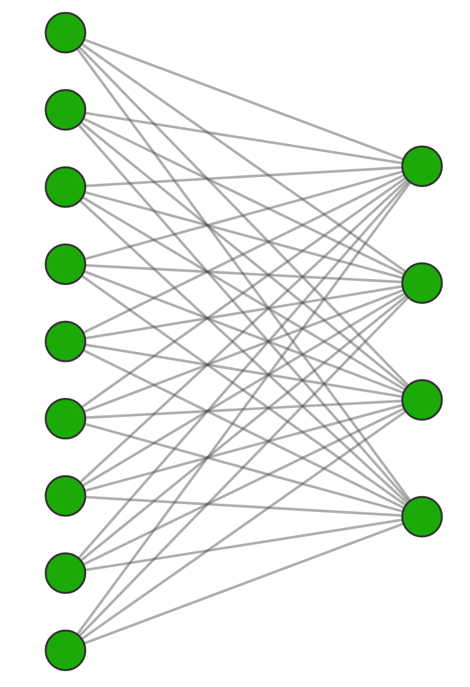
It is instructive to appreciate the relation between general deep learning models, not domain-specific, and CNN which is particularly tailored for computer vision.
Why? because you will better understand frequently-mentioned concepts that are rarely explained well:
- Sparsity of connections
- Parameter sharing
- Hierarchical feature engineering
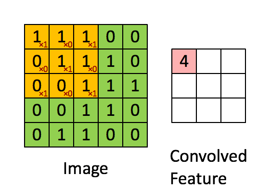
Vectorization will help us here. Vectorize the input matrix, think of each pixel as an individual input. The filter convolves over the matrix, creating what is called a feature map. Vectorize that feature map also. Consider each entry in the feature map as a hidden unit. The example below is as simple as could be, for clarity.
The image matrix is a [3 by 3] and the filter is [2 by 2]. Since the output will be also [2 by 2], after vectorization we have a vector of 4 hidden units denoted {f1, f2, f3, f4}. I enumerated the pixels and colored the weights for clarity. Press play.
Sparsity of connections
While a fully connected layer would have 9 active weights connecting the 9 inputs to each of the hidden unit, here we only have 4 connecting weights. Sparse means thinly scattered or distributed; not thick or dense. So since we only allow for 4, rather than the possible 9, we describe it as sparsity of connections.
Parameter sharing*
The filter has 4 parameters. Those are the same parameters for each of the hidden units – in that sense they share the same value. Hence the somewhat confusing term parameter sharing (sounds like they are sharing pizza). The reason it’s a good idea to share parameters is that if a shape to be learned, it should be learned irrespective of its exact location on the image. We don’t want to train one set of parameters to recognize a cat in the left side of the image, and train another set of parameters to recognize a cat in the right side of the image.
With parameter sharing we can do away with estimating a fully connected layer (36 parameters). Instead, we only estimate 4 parameters. But this is quite restrictive, which is the reason for adding many (say 64) feature maps to retrieve the much-needed flexibility for a good model. This is a nice bridge to hierarchical feature engineering.
Hierarchical feature engineering
The following is taken from the paper Imagenet classification with deep convolutional neural networks. 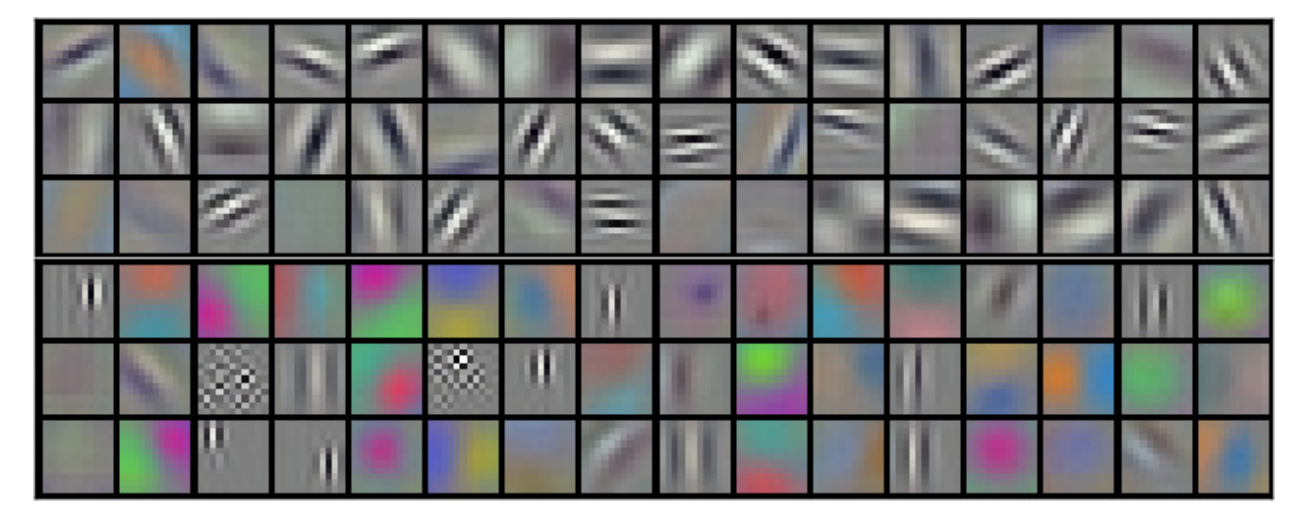
Each small square is a matrix, representing the weights which have been learned by the model. Read it from top to bottom. The top three rows are learned weights\filters early in the network. The bottom three rows are learned weights\filters thereafter, taking their inputs from the top 3 among others.
Parameter sharing is so restrictive that it forces the model to make choices. These choices are directed by the need to minimize the loss function. You can see that weights\filters associated with early layers focus on “primitive” feature engineering. Each (convolutional) layer has very little “weights-budget” due to parameter sharing that the model first picks up orientation and edges, almost completely ignoring colors. Subsequent layers in the network (the bottom three rows showing the weights\filters) once “primitive” features have been learned by earlier layers, are “allowed” to focus on more sophisticated features involving colors.
Why this pattern? because more images are recognized by the “primitive” set, so the network starts there. Once the model is happy with one set of weights, it can move on to minimize the loss further by trying to recognize additional, more complex patterns.Similar observation is made in Convolutional deep belief networks for scalable unsupervised learning of hierarchical representations.
Footnotes and references
Footnotes
* We have seen parameter sharing in the past in the context of volatility forecasting. particularly equation (4) in the paper A Simple Approximate Long-Memory Model of Realized Volatility assign the same AR coefficient for different volatility lags.


