Contents
Introduction
Google “K-means clustering”, and you usually you find ugly explanations and math-heavy sensational formulas*. It is my opinion that you can only understand those explanations if you don’t need them; meaning you are already familiar with the topic. Therefore, this is a more gentle introduction to K-means clustering. Here you will find out what K-Means Clustering, an algorithm, actually does. You will get only the basics, but in this particular topic, the extensions are not wildely different.
Clustering is nothing more than grouping items together based on how similar they are to each other. Similarity is typically filled in by some measure of closeness, or distance. Hence, that is our starting point. Later we apply the K-Means Clustering algorithm to a set of ETFs, grouping them into two categories: risky and less risky.
Distance Calculations
You would think the distance between two numbers should be easy to compute. It i, but you need to define what is it that we call distance. In the physical world, two points are always relative to each other. So London can be 0, and Amsterdam can be 356.67 (Kilometers), or Amsterdam can be 0 and London can be 356.67, but no negative values. In math, we keep the zero as an anchor. So a point can be easily sitting on a negative value. We are often busy with summing up different distances, so it is good if the distances don’t cancel out. So we define a distance in absolute terms:  . This is called Mahalanobis distance. Given that there is a very tight link between this distance measure and our own physical world, you would think that this is the most common distance measure. Not so. We usually prefer to work with something which is called the Euclidean distance:
  . There are couple of advantages for using Euclidean distance, but mainly because it is mathematically agreeable; it is easier to derive and manipulate this measure, so you will see it more often than the Mahalanobis distance. From this point on, here we understand the term “distance” as “Euclidean distance”.
Expanding the dimension from calculating distance between points to calculating distance between vectors is easy. You simply sum up the individual point distances, this is what is behind the dist function in R:
point_a <- t(c(runif(1, 1, 3), runif(1, 1, 3)))
point_b <- t(c(runif(1, 1, 3), runif(1, 1, 3)))
dist(rbind(point_a, point_b))
     1
2 0.706
sqrt( (point_a[1] - point_b[1])^2 + (point_a[2] - point_b[2])^2 )
[1] 0.706
For those you who are right-brain strong, visually it looks like this: 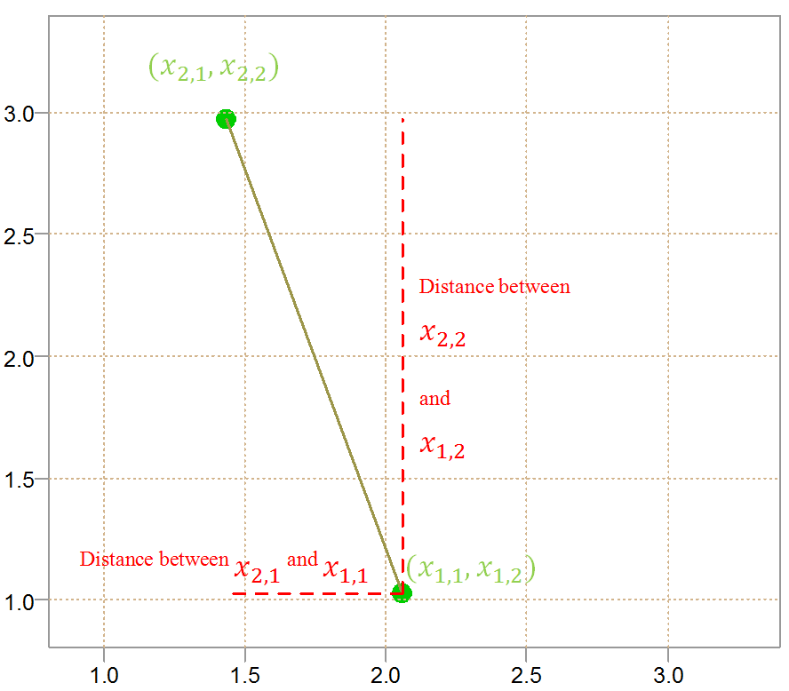
As you can see, the figure has a pleasing pythagorasian feel to it. Higher dimension are complicated to plot, but the principle is the same. You can also appreciate why the math is so crowded when it comes to clustering. We have the points, each point has its coordinates in space, we need to difference, square, square-root and sum over different points with different space coordinates. By the way, those coordinates in space are simply the features, or characteristics or explanatory variable (depends who you ask). Usually the first subscript for the points is denoted by i, and the second subscript for the features is denoted by j. We now know what we need to talk about the K-Means Clustering algorithm.
K-Means Clustering
In order for us to have something specific to talk about, let’s pull some ETF tickers data and try to group them into risky and less risky using K-Means Clustering. The following code pulls and arrange the data into a workable format:
library(quantmod)
citation("quantmod")
k <- 10 # how many years back?
end<- format(Sys.Date(),"%Y-%m-%d")
start<-format(Sys.Date() - (k*365),"%Y-%m-%d")
symetf = c('XLY','XLP','XLE','XLF','XLV','XLI','XLB','XLK','XLU')
l <- length(symetf)
w0 <- NULL
for (i in 1:l){
dat0 = getSymbols(symetf[i], src="yahoo", from=start, to=end, auto.assign = F,
warnings = FALSE, symbol.lookup = F)
w1 <- weeklyReturn(dat0)
w0 <- cbind(w0,w1)
}
time <- as.Date(substr(index(w0),1,10))
w0 <- as.matrix(w0)
colnames(w0) <- symetf
Now w0 is a matrix with weekly returns. We want to group/cluster the ETFs according to risk. First we need to decide on our definition of risk, let’s use volatility and skewness. Ignoring diversification benefits, negative skewness is less risky. The following code compute those characteristics for the different ETFs:
characteristics_names <- c("sd",  "kurtosi") # The latter is from the psych package
characteristics <- characteristics0 <- NULL
for (i in characteristics_names) {
characteristics0 <- apply(w0, 2, i) # yes, you can do it like that
characteristics <- rbind(characteristics0, characteristics)
}
characteristics_dat <- t(characteristics)
colnames(characteristics_dat) <- characteristics_names
characteristics_dat_scaled <- apply(characteristics_dat, 2, scale)
rownames(characteristics_dat_scaled) <- symetf
characteristics_dat_scaled
        sd kurtosi
XLY -0.226  0.1256
XLP -0.140 -1.4431
XLE -0.181  0.8360
XLF  1.765  1.8930
XLV  0.993 -0.8599
XLI -0.943  0.0743
XLB -1.065  0.4644
XLK -1.037 -0.3657
XLU  0.834 -0.7246
Notice that the data is scaled. Echoing factor analysis, we don’t want our clusters to be driven by variables which have high variance, and scaling places all variables on the same footing. We now need to set the number of clusters- the number of groups we would like to end up with. We keep it simple at two groups (two is the k in k-means). There are many (too many) ways to find the number of clusters which is beyond our concern here (see below for a reference). Now, we would like to have 2-centers. Each center will have a group around it. When we use the word center we mean mean (ta daaam), but there are other measures for what in statistical jargon is called “central tendency”, for example the median is also sort of “middle”. So once you understand this post, you directly understand another kind of clustering technique. You guessed it: K-medians clustering.
How would you compute the center of this data? easy, you can compute the average of each column, this would give you a point with two coordinates. What we would like to do is to have two centers (we call those centroids) which are farther away from each other as possible, so as to to best discern between the two groups we want to find. But, how to find those centroids? Enter the machine (learning) (i.e. we have an algorithm for that).
(1) We start with random assignment of the ETFs into two groups. For each group, (2) we compute the centroid. Then, (3) we compute the distance (see previous section) between each point and both centroids. (4) we assign the observation to the group closest to its centroid. (5) Now, the assignment is different, so the old centroids are not valid as they were computed based on the previous assignments, we re-compute the centroids based on the new assignments. (6) We now go back to (3) and do again the same thing, and keep on doing the same thing until the observations “settle”. At some point the observations WILL be assigned already to its closest centroid and no new assignment will be given. What a story… Think you are better off reading the math? at the bottom for your convenience. Since we chose only the 9 ETFs and only 2 features we can see-through the algorithm and how it works. I usually use static images in my posts but due to the dynamic nature of the algorithm we better look at an animation.
The animation below was created using the animation package**. It shows how the algorithm works, looping couple of times using different starting random assignments. I have tried to set the speed such that it is natural to watch, but you can also click on the buttons to hasten or slow it down. UPDATE: if you can’t see the animation this is because your firm might block dropbox access which is needed here. Try from tablet or from home.
As you can see the process is not terribly stable. Different starting point can easily result in a much different grouping. This is discomforting. As Sum and Qiao write in “Stabilized nearest neighbor classifier and its statistical properties” (see references at the bottom):
Stability is an important and desirable property of a statistical procedure. It provides a foundation for the reproducbility and reflects the credibility of those who use the procedure.
In the case of K-means algorithm an ETF can easily end up being classified as risky or less risky based on the initial random assignment. One way to work around this problem by clustering the ETFs few times, each time based on different random starting point. Later we decide which cluster the ETF belong with using majority voting. There are other ways to overcome this instability. This is a live research branch, see the paper mentioned and references therein if you are into it.
Now that we know how the algorithm works, see how easy it is in R:
# nstart means we wou
kmeans_etf = kmeans(characteristics_dat_scaled, centers= 2, nstart = 5, trace=T)
kmeans_etf$cluster

# XLY XLP XLE XLF XLV XLI XLB XLK XLU
#  1   1   1   2   2   1   1   1   2
So now we have our two groups. Remember, if it is not very computationally expensive, you should increase the number of starting points to try and get a stable result. If you would do that, you would find out that XLF is a stand-alone ETF in terms of its risk, as we defined it here. A nice feature of this algorithm is that you need not specify beforehand how many items in each group. This algorithm is so widely used it is now standard in all modern programming languages.
Subjectivity
K-means clustering is what they call unsupervised learning. Accuracy has nothing to do with it – it depends on the characteristics you wish to focus on. There is no right or wrong. The following items can be classified into two groups as follows:
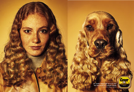

Sure, classifying the two humans together would make more sense perhaps, but those images make a good argument in favour of a different grouping. It all depends on the feature you find important, which links us nicely with possible extensions.
Issues and Extensions
-
1. How do we measure distance for a categorical variables or for ordinal variables? Answered in the The Elements of Statistical Learning book. You can also use other measure of distance which allows for categorical like the Gower Distance.
2. Some points (outliers) can pull the centroid too far for their own good.
3. Do we need all features? Can we ignore features which are less important and how to find those? Those questions along with the previous item are addressed in the
RSKC package (see references).
Appendix (References and mesmerizing math formulas)
- Yumi Kondo, Matias Salibian-Barrera, Ruben Zamar (2016). RSKC: An R Package for a Robust and Sparse K-Means Clustering Algorithm. Journal of Statistical Software
- Will Wei Sun, Xingye Qiao, and Guang Cheng. Stabilized nearest neighbor classifier and its statistical properties. Journal of the American Statistical Association, 111(515):1254–1265,2016
- Yihui Xie (2013). animation: An R Package for Creating Animations and Demonstrating Statistical Methods. Journal of Statistical Software, 53(1), 1-27.
- Data Classification: Algorithms and Applications (link to a book on amazon)
- The K-means algorithm explained in Wikipedia. As I mentioned in the first paragraph, I don’t think it is overly clear but still copy pasted here if you feel like crossing the math with the explanations given above.
1. Assignment step: Assign each observation to the cluster whose mean yields the least within-cluster sum of squares (WCSS). Since the sum of squares is the squared Euclidean distance, this is intuitively the “nearest” mean.[6] (Mathematically, this means partitioning the observations according to the Voronoi diagram generated by the means).![\[S_{i}^{(t)}={\big \{}x_{p}:{\big \|}x_{p}-m_{i}^{(t)}{\big \|}^{2}\leq {\big \|}x_{p}-m_{j}^{(t)}{\big \|}^{2}\ \forall j,1\leq j\leq k{\big \}},\]](https://eranraviv.com/wp-content/ql-cache/quicklatex.com-236308670a8604953d7bee7f0027a7ac_l3.svg "Rendered by QuickLaTeX.com")
where each
 is assigned to exactly one
  , even if it could be assigned to two or more of them.
2. Update step: Calculate the new means to be the centroids of the observations in the new clusters.
![\[{\displaystyle m_{i}^{(t+1)}={\frac {1}{|S_{i}^{(t)}|}}\sum _{x_{j}\in S_{i}^{(t)}}x_{j}}\]](https://eranraviv.com/wp-content/ql-cache/quicklatex.com-fd20e00610b004f0d5669299a6128bde_l3.svg "Rendered by QuickLaTeX.com")
Since the arithmetic mean is a least-squares estimator, this also minimizes the within-cluster sum of squares (WCSS) objective.
*
![\[W(C_k) = \frac{1}{ \vert C_k \vert} \sum_{i, i^{\prime} \in C_k} \sum_{j=1}^p (x_{ij} - x_{i^ {\prime} j} )^2\]](https://eranraviv.com/wp-content/ql-cache/quicklatex.com-b29bad4cb902b273a99f5526ac62dbce_l3.svg "Rendered by QuickLaTeX.com")


Great article; easy for an amateur to follow. Thank you.
Good to hear. You are welcome.
Hello,
Just one thing.. I guess that this language that you’re using (R, I think?) is not very easy to understand. Sorry to say :0
There is some learning to be done there I agree.