Randomized Matrix Multiplication

Matrix multiplication is a fundamental computation in modern statistics. It’s at the heart of all concurrent serious AI applications. The size of the matrices nowadays is gigantic. On a good system it takes around 30 seconds to estimate the covariance of a data matrix with dimensions $X_{10000 \times 2500}$ , a small data today’s standards mind you. Need to do it 10000 times? wait for roughly 80 hours. Have larger data? running time grows exponentially. Want a more complex operation than covariance estimate? forget it, or get ready to dig deep into your pockets.

We, mere minions who are unable to splurge thousands of dollars for high-end G/TPUs, are left unable to work with large matrices due to the massive computational requirements needed; because who wants to wait few weeks to discover their bug.

This post offers a solution by way of approximation, using randomization. I start with the idea, followed by a short proof, and conclude with some code and few run-time results.

Randomized matrix multiplication

Randomization has long been a cornerstone of modern statistics. In the, unfortunately now-retired blog of the great mind Larry Wasserman, you can find a long list of statistical procedures where added randomness plays some role (many more are mentioned in the comments of that post). We randomly choose a subset of rows\columns, and multiply those smaller matrices to get our approximation.

To fix notation, denote $()^{(i)}$ as the ith column and $()_{(i)}$ as the ith row of some matrix A. Then the product $AB$ can be written as

$A B=\sum_{i=1}^n A^{(i)} B_{(i)}$

where $n$ is the column index for A and row index for B. We later code this so it’s clearer.

Say A is $A_{m \times n}$ and B is $B_{n \times k}$ , now imagine both A and B have completely random entries. Choosing say only $d=1$ row\column, calculating the product and multiplying that product by $n$ (as if we did it $n$ times) would provide us with an unbiased estimate for the sum of all $n$ products; even though we only chose one at random. And yes, there will be variance, but it will be an unbiased estimate. Here is a short proof of that.

$\begin{aligned} \mathbb{E}\left[\sum_{t=1}^m \frac{1}{m p_{i_t}} A^{\left(i_t\right)} B_{\left(i_t\right)}\right] & =\sum_{t=1}^m \frac{1}{m} \mathbb{E}\left[\frac{1}{p_{i_t}} A^{\left(i_t\right)} B_{\left(i_t\right)}\right]=\sum_{t=1}^m \frac{1}{m}\left[\sum_{k=1}^d \mathbb{P}\left(i_t=k\right) \frac{1}{p_k} A^{(k)} B_{(k)}\right] \\ & =\sum_{t=1}^m \frac{1}{m}\left[\sum_{k=1}^d p_k \frac{1}{p_k} A^{(k)} B_{(k)}\right]=\sum_{t=1}^m \frac{1}{m}\left[\sum_{k=1}^d A^{(k)} B_{(k)}\right] \\ & =\sum_{t=1}^m \frac{1}{m}[A B] \\ & =A B \end{aligned}$

In the second transition when we lose the expectation operator remember from probability that $E(X) = \sum_{k=1}^d p(X= x_k) x_k$ .

The proof shows that we need the scaling constant $\frac{1}{m p_i}$ for the expectation to hold. It also shows that the product of the two smaller matrices (with number of columns/rows smaller than $n$ ) is the same, in expectation, as the product of the original matrices $AB$ . Similar to how bootstrapping offers an unbiased estimator, this method also provides an unbiased estimate. It is a bit more involved due to its two-dimensional nature, but just as you can sum or average scalars or vectors, matrices can be summed or averaged in the same manner. The code provided below will clarify this.

What do we gain by doing this again? We balance accuracy with computational costs. Selecting only a subset of columns/rows we inevitably sacrifice some precision, but we significantly reduce computing time, so a practical compromise.

The variance of the estimate relative to the true value of AB (obtained through precise computation) can be high. But similar to the methodology used in bootstrapping, we can lesser the variance by repeatedly performing the subsampling process and averaging the results. Now you should wonder: you started doing this to save computational costs, but repeatedly subsampling and computing products of “smaller matrices” might end up being even more computationally demanding than directly computing AB, defeating the purpose of reducing computational costs. Enter parallel computing.

Just as independent bootstrap samples can be computed in parallel, the same principle applies in this context. Time to code it.

Simple demonstration

I start with a matrix $X_{T \times P}$ with dimension $200 \times 50$ . I then compute the actual $X^ \prime X$ because I want to see what is the difference and how good is the approximation. We base the approximation on quarter of the number of rows TT/4. We vectorize the diagonal and off-diagonal entries (because $X ^ \prime X$ is symmetric) and examine the difference between the actual result and the approximated result.


TT <- 200
p <- 50
A <- do.call(cbind, lapply(rep(TT,p), rnorm) ) 

mult_actual <- t(A) %*% A # Target
vec_actual <- mult_actual[upper.tri(mult_actual, diag= T)]

length(vec_actual) # (P/2) \times (P-1) + P, for the diagonal

m <-  TT/4 # only quarter of the number of rows
 mult_approx_array <- array(dim= c(rr, dim(mult_actual)) )
for (i in 1:rr) {
tmpind <- sample(1:TT, m, replace = T)
mult_approx_array[i,,] <- t(A)[,tmpind] %*% A[tmpind,]
}
# Now average the matrices across rr "bootstrap samples"
mult_approx <- (TT/m) * apply(mult_approx_array, c(2,3), mean) 
# The scaling constant TT/m is because we sample uniformly 
# so each row is chosen with prob 1/TT.
# The eventual approximation (individual entries):
vec_approx <- mult_approx[upper.tri(mult_approx, diag= T)] 
# Difference
vec_diff <- (vec_actual - vec_approx)
plot(vec_diff)

TT <- 200

p <- 50

A <- do.call(cbind, lapply(rep(TT,p), rnorm) )

mult_actual <- t(A) %*% A # Target

vec_actual <- mult_actual[upper.tri(mult_actual, diag= T)]

length(vec_actual) # (P/2) \times (P-1) + P, for the diagonal

m <- TT/4 # only quarter of the number of rows

mult_approx_array <- array(dim= c(rr, dim(mult_actual)) )

for (i in 1:rr) {

tmpind <- sample(1:TT, m, replace = T)

mult_approx_array[i,,] <- t(A)[,tmpind] %*% A[tmpind,]

}

# Now average the matrices across rr "bootstrap samples"

mult_approx <- (TT/m) * apply(mult_approx_array, c(2,3), mean)

# The scaling constant TT/m is because we sample uniformly

# so each row is chosen with prob 1/TT.

# The eventual approximation (individual entries):

vec_approx <- mult_approx[upper.tri(mult_approx, diag= T)]

# Difference

vec_diff <- (vec_actual - vec_approx)

plot(vec_diff)

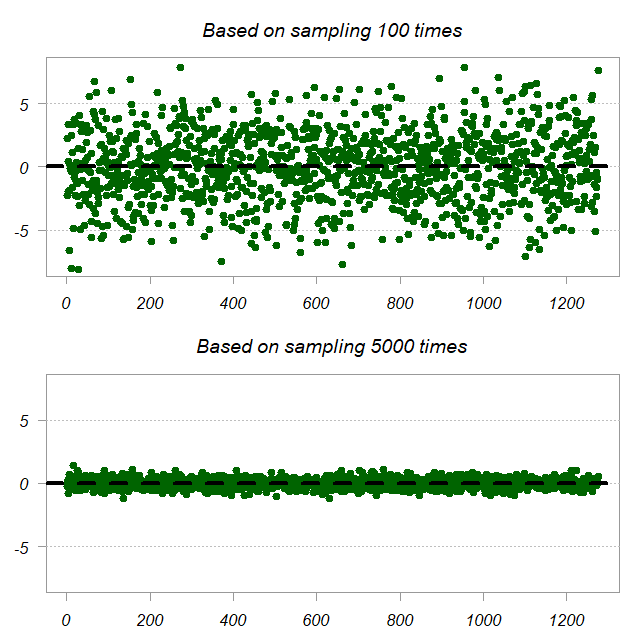
We have 1275 unique entries (off diagonal and diagonal of $X^ \prime X$ ). Each such entry has the approximated value and the true value, we plot the difference. Top panel shows the difference when we average across 100 subsamples and the bottom is based on 5000 subsamples, so of course it’s more accurate.

Let’s talk business

Below is a more production-ready code, for when you actually need to work with big matrices. It parallels the computation using the parallel package in R.


 TT <- 10000
 p <- 2500
 A <- do.call(cbind, lapply(rep(TT,p), rnorm) ) 
 dim(A)
[1] 10000  2500
 m <- TT/4
 
# How long to get exact solution?
 system.time ( t(A) %*% A )
   user  system elapsed 
     30       0      30  # 30 seconds

# Let's apply the following function using a built-in optimized approach 
# we use rr=5 samples for now
tmpfun <- function(index){
  tmpind <- sample(1:TT, m, replace= T)
 (TT/m)*(t(A)[,tmpind] %*% A[tmpind,])
}

rr <- 5 

system.time ( mult_approx_array <- lapply(as.list(1:rr), tmpfun) )
   user  system elapsed 
  37.45    0.28   37.75  # so doing it 5 times takes 37 seconds

# Now in parallel 
library(parallel)
numCores <- detectCores() / 2  # Using half of the available cores
cl <- makeCluster(numCores)
clusterExport(cl, varlist = c("A", "TT", "m") )
system.time ( mult_approx_array_par <- parLapply(cl, 1:rr, tmpfun) )

# The equalizer clicks his suunto watch:
user  system elapsed 
0.20    0.12   13.27 # 13 seconds

stopCluster(cl)

TT <- 10000

p <- 2500

A <- do.call(cbind, lapply(rep(TT,p), rnorm) )

dim(A)

[1] 10000 2500

m <- TT/4

# How long to get exact solution?

system.time ( t(A) %*% A )

user system elapsed

30 0 30 # 30 seconds

# Let's apply the following function using a built-in optimized approach

# we use rr=5 samples for now

tmpfun <- function(index){

tmpind <- sample(1:TT, m, replace= T)

(TT/m)*(t(A)[,tmpind] %*% A[tmpind,])

}

rr <- 5

system.time ( mult_approx_array <- lapply(as.list(1:rr), tmpfun) )

user system elapsed

37.45 0.28 37.75 # so doing it 5 times takes 37 seconds

# Now in parallel

library(parallel)

numCores <- detectCores() / 2 # Using half of the available cores

cl <- makeCluster(numCores)

clusterExport(cl, varlist = c("A", "TT", "m") )

system.time ( mult_approx_array_par <- parLapply(cl, 1:rr, tmpfun) )

# The equalizer clicks his suunto watch:

user system elapsed

0.20 0.12 13.27 # 13 seconds

stopCluster(cl)

Couple of comments are in order. First, if you look carefully at the code, the function tmpfun takes an unnecessary, fictitious index argument which is never used. It has to do with the cluster’s internal mechanism which needs an element to pass on as an argument. Second, the computational complexity in this case is $\mathcal{O}(\#rows^2 \times \#columns)$ , so you can expect larger computational time gains for longer matrices. Third and finally, we sampled rows uniformly (therefore $prob_{row_i} = \frac{1}{TT}$ ). This is primitive. There are better sampling schemes not covered here which will reduce the variance of the result.