Correlation and Correlation Structure (6)

While linear correlation (aka Pearson correlation) is by far the most common type of dependence measure there are few arguably better ways to characterize\estimate the degree of dependence between variables. This is a fascinating topic I keep coming back to. There is so much for a typical geek to appreciate: non-linear dependencies, should we consider the noise in the data or rather just focus on the underlying process, should we consider the whole distribution or just few moments.

In this post number 6 on correlation and correlation structure I share another dependency measure called “distance correlation”. It has been around for a while now (2009, see references). I provide just the intuition, since the math has little to do with the way distance correlation is computed, but rather with the theoretical justification for its practical legitimacy.

Denote $\mathcal{R}(X, Y)$ as the distance correlation. The following is taken directly from the paper Brownian distance covariance (open access) :

Our proposed distance correlation represents an entirely new approach. For all distributions with finite first moments, distance correlation R generalizes the idea of correlation in at least two fundamental ways:

$\mathcal{R}(X, Y)$ is defined for X and Y in arbitrary dimension.

$\mathcal{R}(X, Y) = 0$ characterizes independence of X and Y.

The first point is super useful and far from trivial. You can theoretically calculate distance correlation between two vectors of different lengths (e.g. 12 monthly rates and 250 daily prices)^*. The second is a must-have for any aspiring dependence measure. While linear correlation be computed to be very small number even if the vectors are dependent or even strongly dependent (quite easily mind you), distance correlation is general enough so that when it’s close to zero, then the vectors must be totally independent (linearly and non-linearly).

Although they don’t present it like this in the paper, the idea is a simple functional extension of a usual probabilistic fact: if two random variables are independent then

$P(X=a \text { and } Y=b)=P(X=a) \cdot P(Y=b)$

Now instead of thinking about variables, think about X and Y as functions (in the paper they use characteristic functions), X and Y are independent if and only if

$f_{X, Y}=f_{X} f_{Y}$

Now you can quantify how far the joint function $f_{X, Y}$ is from the product of the two individual functions $f_{X} f_{Y}$ . If they are identical, the distance will be zero. Use the complement [1 – 0] to get a measure that returns 1 for full dependency and 0 for complete independence. It’s a bit like saying the following: if $P(A) = P(B) = 0.5$ , and $P(X=a \text { and } Y=b)= 0.3$ while if they are independent I expect $P(X=a \text { and } Y=b)= 0.25,$ ( $0.5 \times 0.5 = 0.25$ ), then $(0.3-0.25 = 0.05)^2$ is my measure for how dependent are those random variables. Informally speaking we can say we compute some sort of “excess dependency over the fully independent case”. We have seen this idea before talking about asymmetric correlations of equity portfolios.

I replicated figure (1) from the previous post on this topic and I add the distance correlation measure (denoted here as $\widehat{\nu}$ ) for comparison. Afterwards we can say a few words about advantages or disadvantages.

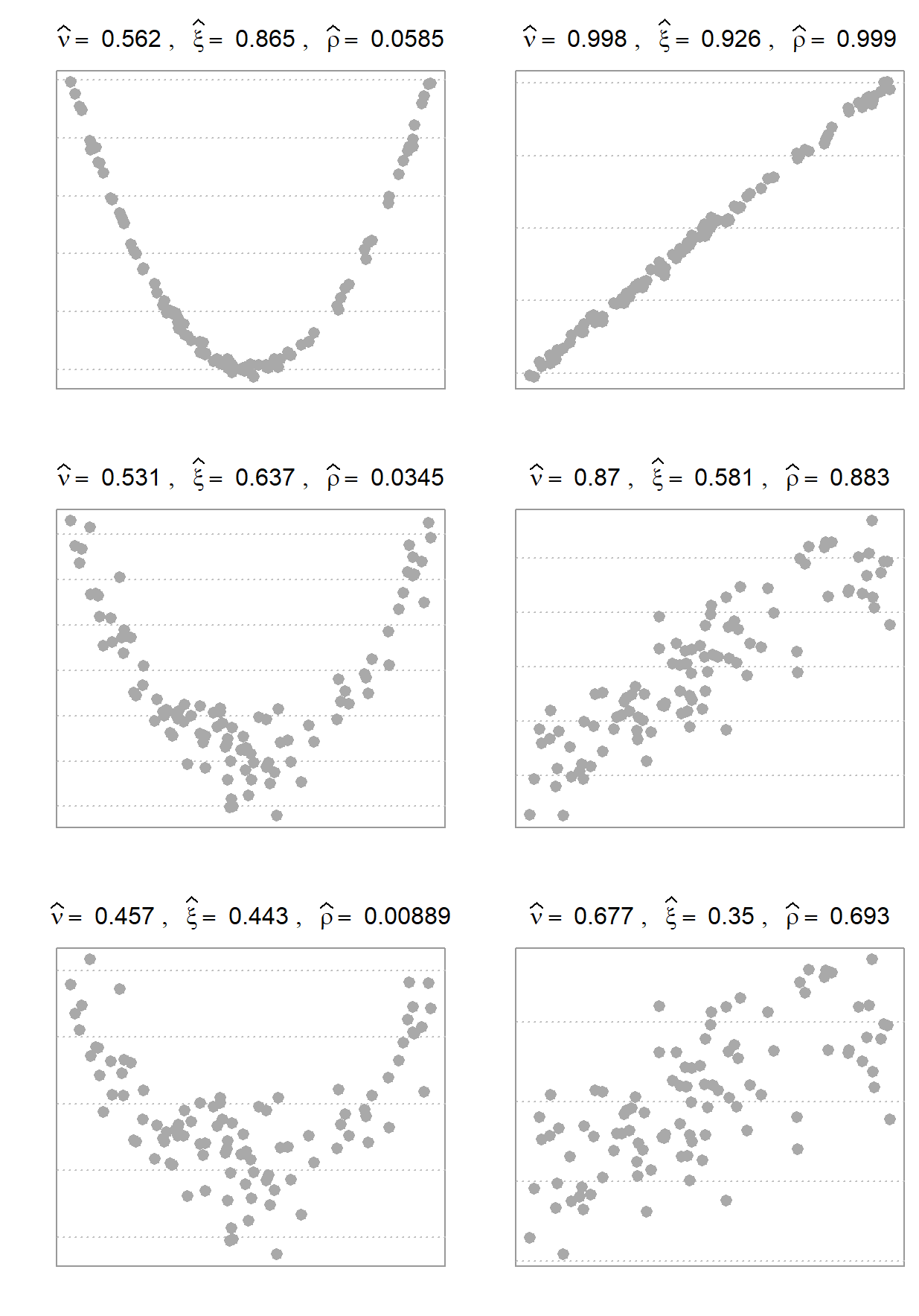
$\widehat{\nu}$ denotes distance correlation, $\widehat{\xi}$ denotes the “new coefficient of correlation” (as they dub it in the original paper), and $\widehat{\rho}$ denotes the usual Pearson correlation. Distance correlation measure relies on the characteristic functions of the realized vectors (think simply their probability distribution). Therefore it cares about the profile of dependence, rather than the strength of dependence; which is the main takeaway from the figure. By way of contrast you see that “new coefficient of correlation” $\widehat{\xi}$ dramatically decreases (from top to bottom) as noise being added to the data. Distance correlation is less sensitive to that. The following figure offers some clarity, I hope:

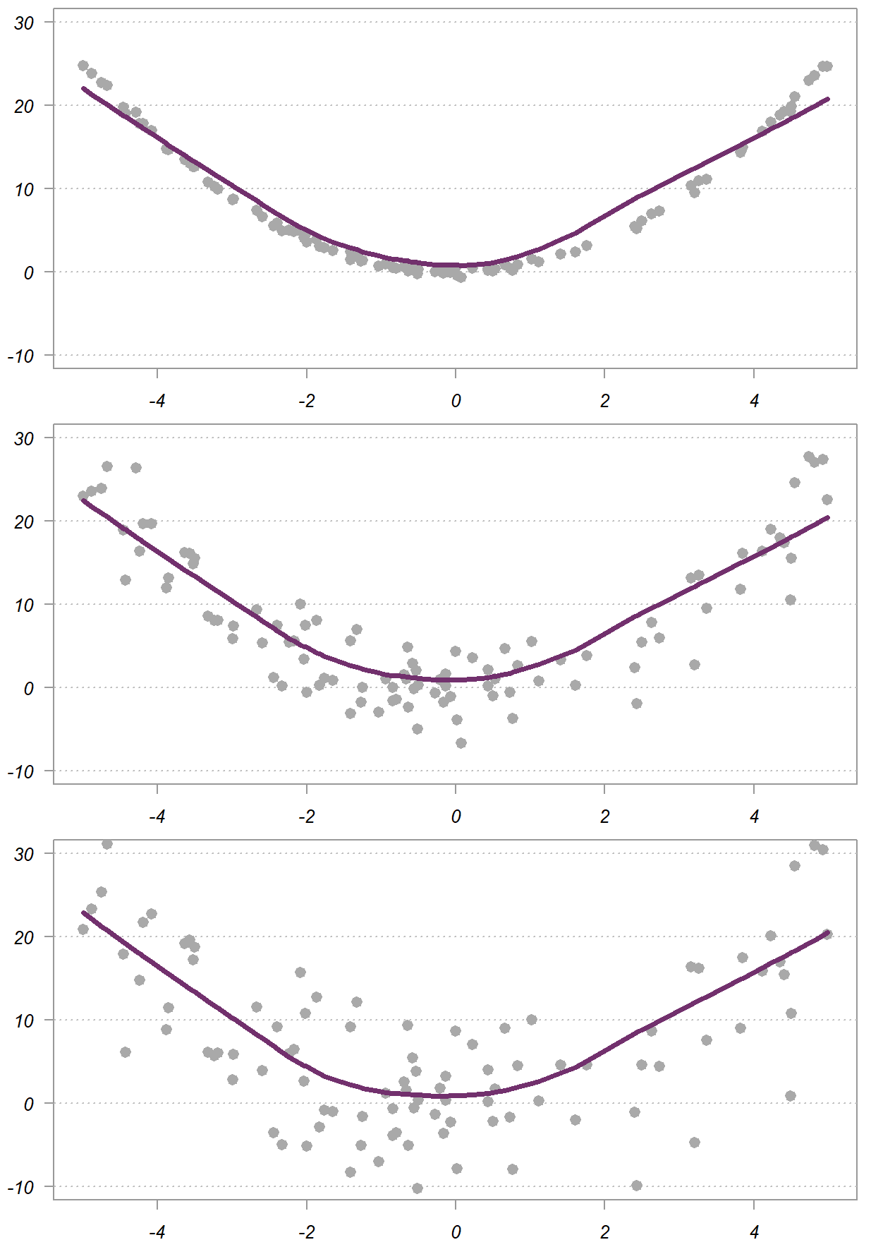
Regardless of the added noise – from top to bottom in the figure, the relation between the two variables x and y, depicted using the purple smooth line, is very similar. The dependency value for the $\xi$ measure is decidedly decreasing as noise being added, because it also considers the noise in the data, while distance correlation focuses on the underlying dependency structure, only.

So, you decided to use a dependency measure that captures both linear and non-linear dependence.

Should you then use $\xi$ , or $\nu$ ?

It’s a matter of preference.

If the empirical realization is what matters to you – meaning you would like to account for the noise in the data, the $\xi$ measure is the way to go. If what you care about is the underlying “skeleton profile” then you should opt for using distance covariance\correlation.

Correlation between stocks and bonds, again..

Correlation between stocks and bonds is an interesting case in point. These two are undoubtedly correlated, but with a complicated dependence structure which has to do with the economy and anticipated actions by central banks. Let’s see what the three dependency measure report for two relevant tickers: TLT (long term US bong ETF) and SPY (S&P 500 ETF). I also plot an estimated smoother for the two time series (in green).

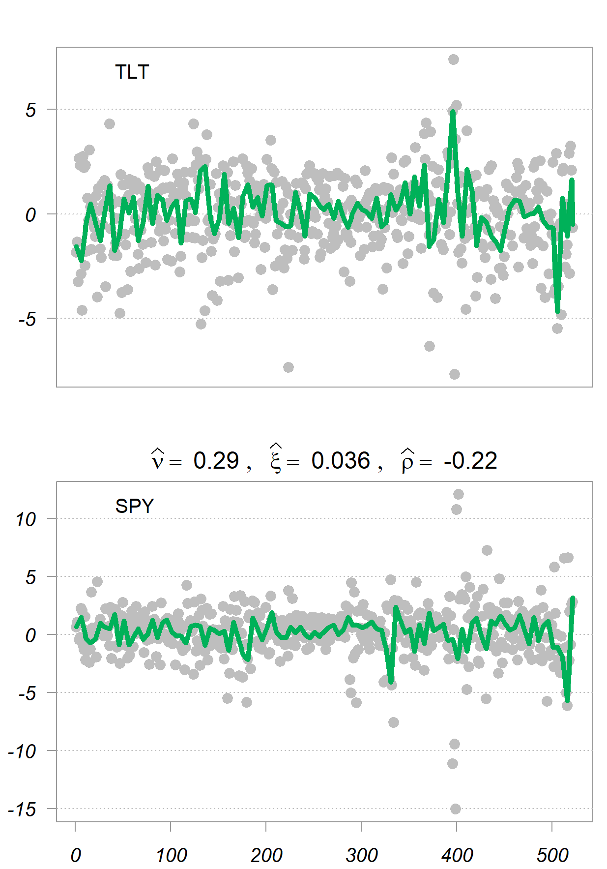
Interesting stuff. We observe that:

Linear correlation $\widehat{\rho}$ is negative, which makes sense on the whole.

$\widehat{\xi}$ is close to zero given that the return series are super noisy

Distance correlation tells of quite a strong dependency between the two series.

You may wonder about the sign, but remember that both $\widehat{\xi}$ and distance correlation are tailored to capture also non-linear dependencies, which makes the sign irrelevant (they both range between 0 and 1).

References

Székely, Gábor J., and Maria L. Rizzo. “Brownian distance covariance.” The annals of applied statistics 3, no. 4 (2009): 1236-1265.

Chatterjee, Sourav. “A new coefficient of correlation.” Journal of the American Statistical Association 116, no. 536 (2021): 2009-2022.

Ang, Andrew, and Joseph Chen. “Asymmetric correlations of equity portfolios.” Journal of financial Economics 63, no. 3 (2002): 443-494. Here for a working-paper version.

Footnotes

* That said, I only found implementations that allow for equal vector length. But you can code it if you need.

You might also like:

2 comments on “Correlation and Correlation Structure (6) – Distance Correlation”

Pingback: Quantocracy's Daily Wrap for 08/15/2022 - Quantocracy
Tomas says:

09/21/2022 at 5:12 PM

Super interesting read! From the concluding figure, one could say that the question of whether to use the “new coefficient of correlation” or the distance correlation boils down to the amount of noise in the data. If the former is close to 0, it seems worthwhile to check whether the latter one is 0 as well. If it is not, then there might actually be some dependence between the variables, but the noise is concealing it from the “new coefficient of correlation”.

Correlation between stocks and bonds, again..

References

You might also like:

2 comments on “Correlation and Correlation Structure (6) – Distance Correlation”

Leave a Reply to Tomas