Last time we showed how to estimate a CCC and DCC volatility model. Here I describe an advancement labored by Engle and Kelly (2012) bearing the name: Dynamic equicorrelation. The idea is nice and the paper is well written.
Departing where the previous post ended, once we have (say) the DCC estimates, instead of letting the variance-covariance matrix be, we force some structure by way of averaging correlation across assets. Generally speaking, correlation estimates are greasy even without any breaks in dynamics, so I think forcing some structure is for the better.
In essence, the authors propose to let:
(1)
where denotes the n-dimensional identity matrix, in our case with 3 ETFs:
and
is in our case
matrix of ones. Convince yourself that this is nothing more than fixing the free off-diagonal elements of
at some restricted value
It is of course natural to choose this value to be the average cross correlation at each point in time.
Demonstration
We use the same assets from last time. We fit a DCC model and proceed to fix the off-diagonal entries at their cross sectional average. Last time we used the univariate garch package rugarch for illustration purposes, but since the focus is now progressed we will use the quicker multivariate rmgarch package.
|
1 2 3 4 5 6 7 8 9 10 11 12 13 14 15 16 17 18 19 20 21 22 23 24 25 26 27 28 29 30 31 32 33 34 35 36 |
library(quantmod) library(rugarch) library(rmgarch) # Pull the data k <- 10 # how many years back? end<- format(Sys.Date(),"%Y-%m-%d") end_training <- "2015-01-01" start<-format(Sys.Date() - (k*365),"%Y-%m-%d") sym = c('SPY', 'TLT', 'IEF') l <- length(sym) dat0 = getSymbols(sym[1], src="yahoo", from=start, to=end, auto.assign = F, warnings = FALSE, symbol.lookup = F) n = NROW(dat0) dat = array(dim = c(n,NCOL(dat0),l)) ; ret = matrix(nrow = n, ncol = l) for (i in 1:l){ dat0 = getSymbols(sym[i], src="yahoo", from=start, to=end, auto.assign = F, warnings = FALSE, symbol.lookup = F) dat[1:n,,i] = dat0 ret[2:n,i] = (dat[2:n,4,i]/dat[1:(n-1),4,i] - 1) # returns, close to close, percent } ret <- 100*na.omit(ret)# Remove the first observation time <- index(dat0)[-1] colnames(ret) <- sym nassets <- dim(ret)[2] TT <- dim(ret)[1] # Fit a ghreshold garch process gjrtspec <- ugarchspec(mean.model=list(armaOrder=c(0,0)), variance.model =list(model = "gjrGARCH"),distribution="std") # dcc specification - GARCH(1,1) for conditional correlations dcc_spec = dccspec(uspec = multispec(replicate(l, gjrtspec)), distribution = "mvt") # Fit DCC garchdccfit = dccfit(dcc_spec, ret, fit.control=list(scale=TRUE)) # print(garchdccfit) # If you want to see the information - parameters etc. slotNames(garchdccfit) # To see what is in the object names(garchdccfit@model) # To see what is in the object names(garchdccfit@mfit) # To see what is in the object # plot(garchdccfit) # All kind of cool plots |
What is important now is to get the covariance over time, so as to build a portfolio. We can extract an array of size from the object garchdccfit, which means the covariance matrix in the 3 by 3 matrix, over time in the third dimension:
|
1 2 3 4 5 6 7 |
dcccov=rcov(garchdccfit) # for covariance dcccor=rcor(garchdccfit) # for correlation dim(dcccor) [1] 3 3 2514 mean_rho <- apply(cbind(dcccor[1,2,], dcccor[1,3,], dcccor[2,3,]),1,mean) # for later |
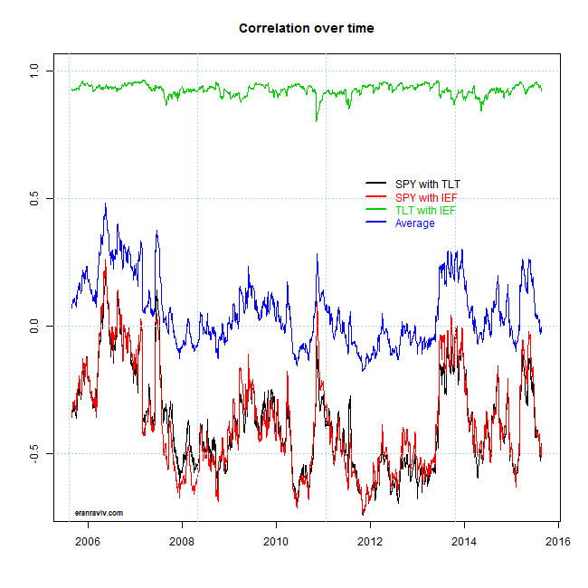
What we do now is have a look how the correlation evolves over time, and how the average of those correlation looks over time:
 We see the correlation between the two fixed-income ETFs is extremely high and quite stable. The correlation with the SPY is less so, shifting between 0 and quite negative. The image is very much related to the correlation-structure post. We see how recently, with the increased volatility in the market, we have moved quickly to negative correlation region. What is nice about looking at correlations is that from simply looking at series themselves you may not realize this is happening. I mean, it is not like SPY is tanking while TLT is booming. We can here see it more clearly since in the computation, correlation considers the volatility of TLT. Meaning to say that fixed income does not need to boom in order to provide the diversification benefits it is supposed to provide.
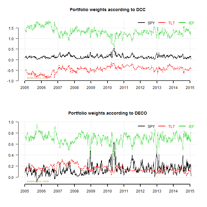
The blue line is simply the average of the other three lines. At each time point, instead of letting each entry in the covariance matrix be free, we can set it to the value in the blue line. The next few lines construct a portfolio from two different estimation of the covariance matrix. The one is the DCC, and in the other we use the idea promoted by Engle and Kelly. After that we will plot the weights of the two different portfolios, aimed to minimize volatility of the portfolio.
|
1 2 3 4 5 6 7 8 9 10 11 12 13 14 15 |
mu <- apply(ret,2,mean) # mean daily returns wdcc <- wdeco <- matrix(nrow = TT, ncol = nassets) # make room for portfolio weights dec_cov <- array(dim = c(nassets,nassets,TT)) # make room for the covariances of DECO for (i in 1:TT){ # The function globalMin.portfolio can be found here: http://faculty.washington.edu/ezivot/econ424/portfolio.r wdcc[i, ] <- globalMin.portfolio(252*mu, dcccov[,,i])$weights dt <- sqrt(dcccov[,,i]*diag(nassets)) eq_cor <- diag(nassets) eq_cor[upper.tri(eq_cor,diag=F)] <- mean_rho[i] eq_cor[lower.tri(eq_cor,diag=F)] <- mean_rho[i] dec_cov[,,i] <- dt %*% eq_cor %*% dt wdeco[i, ] <- globalMin.portfolio(252*mu, dec_cov[,,i])$weights } |

– It looks as if the weights based on DECO covariance are more volatile, but they are less so (mind the Y-scale).
– Weights have become more balanced, with less extreme shorts. This is an important insight. We can apply this shrinkage idea to accomplish a long only portfolio in a smart way, other than optimize under some constraints.
– Note how the weight of the SPY have decreased and the weight of the IEF has increased, as expected given recent events.
——————————————————-
This is the most vanilla implementation possible, here only to fix the idea. The first thing you can think of is to set only part of the entries of the covariance matrix, not all of them as we have done here. I can imagine that fixing all entries when you construct a portfolio of 1K assets is idiotic, but limiting entries according to clusters (industries?) should be useful. As a final note, why the average ? other correlation measures, even based on some side-analysis may provide further refinement.
Code for plots
|
1 2 3 4 5 6 7 8 9 10 11 12 13 14 15 |
par(mfrow = c(2,1), las = 1, bty = "n") matplot(y = wdcc, ty = "l", xaxt="n", xlab="", ylab="") mm <- 250 seqq <- seq(1, TT, mm) axis(side= 1, at = seqq, labels=substr(time,1,4)[seqq], lwd = 2) grid() legend("topright", sym, col = 1:nassets, lty=1, lwd = 2, text.col = 1:nassets, bty = "n", ncol = 3) title("Portfolio weights according to DCC") matplot(y = wdeco, ty = "l", xaxt="n", xlab="", ylab="") axis(side= 1, at = seqq, labels=substr(time,1,4)[seqq], lwd = 2 ) grid() legend("topright", sym, col = 1:nassets, lty=1, lwd = 2, text.col = 1:nassets, bty = "n", ncol = 3) title("Portfolio weights according to DECO") |
References and further readings


Hi, Where do you define the ‘mean_rho()’ function in your R code?
mean_rhois not a function. It is the average correlation. This is the number we shrink towards.Hi Eran,
Did you assume the equicorrelation structure in the example R codes? Thanks.
Yongli
Consider equicorrelation as a add-on structure over your covariance\correlation matrix estimate.
dcccovis without the additional quicorrelation structure while in this line of code:dec_cov[,,i] <- dt %*% eq_cor %*% dtwe force this structure.Hi Eran,
How do you deal with the missing values? If I have the data already, Is it necessary to convert the data to the same class (“xts” “zoo”)?
Thank you.
Personally speaking, I don’t like to convert objects outside the base package (so I try to keep data.frame and matrix as my classes). It is not necessary to convert to xts in order to run the code.
Regarding missing values. You can interpolate them (yourself, using a built-in
approxfunction or use one of the excellent imputation packages available (Ameliacomes to mind) for good NAs interpolation.Hello Eran,
Would you mind sharing the codes for plotting the “correlation over time” graph?
Thanks.
Hi Eran,
Great post. I’ve tried to run your code and it keeps returning:
Error in dat[1:n, , i] <- dat0 :
number of items to replace is not a multiple of replacement length
Do you know why this might be? Sorry, I'm very new to R.
Many thanks
Make sure
nequals NROW(dat0).dat[1:n, , i]is a matrix. Number of rows is n, number of columns is exactly as the number of columns indat0.Dear Professor,
Why do you choose armaOrder=c(0,0)?
According to your comment, your intention is GJR GARCH(1,1).
Anyway, what are the typical armaOrder for fitting stock market, say 212 of S’&P500 stocks (1993-1-1~1996-1-1)?.
gjrtspec <- ugarchspec(mean.model=list(armaOrder=c(0,0)), variance.model =list(model = "gjrGARCH"),distribution="std")
# dcc specification – GARCH(1,1) for conditional correlations