The total nonfarm payroll accounts for approximately 80% of the workers who produce the GDP of the United States. Despite the widely acknowledged fact that the Nonfarm payroll is highly volatile and is heavily revised, it is still driving both bonds and equity market moves before- and after it is published. The recent number came at a weak 142K compared with around 200K average over the past 12M. What we wish we would know now, but will only know later, is whether this number is a start of a weaker expansion in the workforce, or not.
Despite the fact that it is definitely on the weak side (as you can see in the top panel of the figure), it is nothing unusual (as you can see in the bottom panel of the figure).
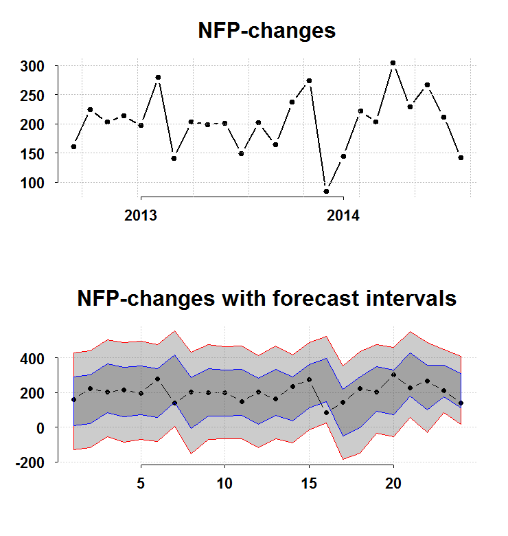
The bottom panel charts the interval you have before the number is publish (forecast intervals) from a simple AR(1) model without imposing normality. The blue and the red lines are 1 and 2 standard deviations respectively. The recent number barely scratches the bottom blue, so nothing to suggest a significant shift from a healthy 200K. On the other hand, there is some persistence:
ar.ols(na.omit(nfp))

Call:
ar.ols(x = na.omit(nfp))

Coefficients:
      1        2        3        4        5        6
 0.2633   0.2672   0.1402   0.0841   0.1015  -0.0853

Intercept: 0.318 (5.906)

Order selected 6  sigma^2 estimated as  31430
So, on average we can expect to trend lower.
Code for figure:
library(quantmod)
library(Eplot)

tempenv <- new.env()
getSymbols("PAYEMS",src="FRED",env=tempenv)
# Bring it to global env
head(tempenv$PAYEMS)
time <- index(tempenv$PAYEMS)
nfp <- as.numeric(diff(tempenv$PAYEMS))
par(mfrow = c(2,1))
k = 24
args(plott)
plott(tail(nfp,k),tail(time,k),return.to.default = F,main="NFP-changes")
args(FCIplot)
nfpsd <- FCIplot(nfp,k=k,rrr1="Rol",rrr2="Rol",main="NFP-changes; forecast intervals superimposed")
 , depends on your initial assumptions, so F-test or
  and we want to get a ‘smaller’ matrix
  with
with  . We want the new ‘smaller’ matrix to be close to the original despite its reduced dimension. Sometimes we say ‘such that Z capture the bulk of comovement in X. Big data technology is such that nowadays the number of cross sectional units (number of columns in X) P has grown to be very large compared to the sixties say. Now, with ‘google maps would like to use your current location’ and future ‘google fridge would like to access your amazon shopping list’, you can count on P growing exponentially, we are just getting started. A lot of effort goes into this line of research, and with great leaps.