Similarity and Dissimilarity Metrics

In the field of unsupervised machine learning, similarity and dissimilarity metrics (and matrices) are part and parcel. These are core components of clustering algorithms or natural language processing summarization techniques, just to name a couple.

While at first glance distance metrics look like child’s play, the fact of the matter is that when you get down to business there are a lot of decisions to make, and who likes that? to make matters worse:

Theoretical guidance is nowhere to be found
Your choices and decisions matter, in the sense that results materially change

After reading this post you will understand concepts like distance metrics, (dis)similarity metrics, and see why it’s fashionable to use kernels as similarity metrics.

Basic similarity metrics

A couple of dissimilarity metrics that you are familiar with: Euclidean distance and Manhattan distance. Since both are special cases of Minkowski distance we briefly only write that one:

$D(X, Y)=\left(\sum_{i=1}^{k}\left|x_{i}-y_{i}\right|^{p}\right)^{\frac{1}{p}}$

Consider D(X,Y) as the “proximity score” for observation $X$ and observation $Y$ . Think about $X$ as an average observation (say an average house with $k$ characteristics), and $Y$ as some other observation. If $p=2$ we have the Euclidean distance, if $p=1$ we have the Manhattan distance. We could determine how far a house is from the average house based on either of those distance metrics. Wonderful, but what is the meaning? which one should we use?

To build some intuition around this question, you can think of a house at the heart of any major city. It’s enough to step out to the suburbs for a serious price drop. So for that kind of reality the Euclidean distance would be more reasonable than the Manhattan distance; a larger exponent for a sharper decrease.

The whole, and only difference between various (dis)similarity metrics is their profile: what is the rate of decline in the “proximity score” as you move the two observations apart, how fast of an increase we observe in the “proximity score” as we move the two observations closer together.

This is one junction where the rubber meets the road. Say you are busy with clustering, the ideal metric is somewhat funky. You want those observations that bunched together to score real close. But if an observation is not close enough (so outside the cluster), then you want that observation to score as far away as possible. In sharp contrast to classical machine learning textbooks, since real data looks different at different regions, finding an intelligent similarity metric is a far cry from a one-size-fits-all situation.

Additional point here before we look at some different profiles of similarity metrics. While we don’t often see Manhattan distance in practice, echoing our previous real-estate example, when our data has large cross-sectional dimension – many columns compared with the number of rows, the higher the $p$ in the formula, the more meaningless the metric becomes. For large and wide data matrix you want to lower the exponent (see here for details and an illustration).

Basic similarity metrics – illustration

The data I use for this post is the Boston housing dataset. We start by scaling the data such that all characteristics (crime rate, number of rooms etc) are on equal footing. We look at the average house, and our aim is to quantify how different each house is, from that average house. The quantification will involve of course a distance measure. We start with the Euclidean distance and the Manhattan distance.

Coding:


library(MASS)
# Boston %>% head
TT <- NROW(Boston)
dat <- Boston %>% scale 

mh <- rep(0, NCOL(dat)) # mh for mean house
dist_mh_manhat <- dist_mh_euclid <- NULL
for (i in 1:TT){
  dist_mh_euclid[i] <- sqrt( sum( (mh - dat[i,])^2 ) )
  dist_mh_manhat[i] <-  sum( abs(mh - dat[i,]) ) 
}

tmp1 <- (1000*dist_mh_euclid/sum(dist_mh_euclid)) %>%  sort
tmp2 <- (1000*dist_mh_manhat/sum(dist_mh_manhat)) %>% sort
plot(tmp1 ~ tmp2, pch= 19, ylab="Euclidean", xlab= "Manhattan")
abline(a=0,b=1, lwd=2, lty= "dashed")

library(MASS)

# Boston %>% head

TT <- NROW(Boston)

dat <- Boston %>% scale

mh <- rep(0, NCOL(dat)) # mh for mean house

dist_mh_manhat <- dist_mh_euclid <- NULL

for (i in 1:TT){

dist_mh_euclid[i] <- sqrt( sum( (mh - dat[i,])^2 ) )

dist_mh_manhat[i] <- sum( abs(mh - dat[i,]) )

}

tmp1 <- (1000*dist_mh_euclid/sum(dist_mh_euclid)) %>% sort

tmp2 <- (1000*dist_mh_manhat/sum(dist_mh_manhat)) %>% sort

plot(tmp1 ~ tmp2, pch= 19, ylab="Euclidean", xlab= "Manhattan")

abline(a=0,b=1, lwd=2, lty= "dashed")

Result:

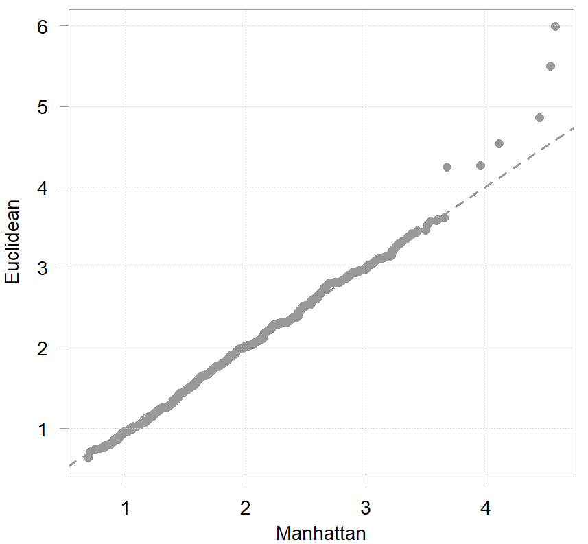
I normalized and multiplied the distances by 1000 for better readability. What is plotted is the sorted relative distances for each house from the average house. The two metrics coincide for all but a handful of houses. That is probably a result of our choice to uniformly standardize the columns of the data matrix. In practice you must also think if all your variables (columns) are “born equal” so to speak.

Now, these are distances, so dissimilarities. If we would compute all pairwise distances we would have a dissimilarity matrix. How do we get from dissimilarity to similarities? how similar two observations are versus how dissimilar two observations are, is this the same question? We know how far each house from the average house is, in terms of (scaled) characteristics. Would be nice to get values between 0 and 1. Ideally an index-like value for how similar two houses are, whereby if they are identical we have a value of 1 and if they are completely different we have the value close to zero. What can we do?

We can apply $f(x) = 1 - x$ , with $x = \frac{distance}{sum(distances)}$
We can apply a different function which reverses the relation between distance and the proximity score

Enter Kernel functions

Kernel functions are continuous, symmetric and positive everywhere. There are many of those functions around, but let’s here talk about just one: the Gaussian kernel. Extensions to other kernels are trivial once you get the concept. In moving from distances (dissimilarities) to similarities, you can think about the Gaussian kernel as a particular function which reverses the relation between the distance and the proximity score (the higher the distance the lower the proximity score). The Gaussian kernel function (with the same notation as above) takes the form

$K\left(\mathbf{X}, \mathbf{Y}\right)=\exp \left(-\frac{\left\|\mathbf{X}-\mathbf{Y}\right\|^{2}}{2 \sigma^{2}}\right) = \exp \left( {-\frac{D(X,Y)}{2 \sigma^{2}} } \right),$

with a $p=2$ in the $D$ metric. Such a function makes sense. Why?

If the distance $D$ is zero, we have an identity and the proximity score is 1. On the other side, if the $D$ is large we get something close to zero.
Profile-wise, it is well to drop the score quickly to zero with increased distance $D$ . So for example, if you live far from the center it matters very little if you need to commute 90 minutes or 100 minutes. It matters much less than the difference between commuting 5 minutes or 15 minutes.
Not only the profile of the function makes sense, but the Gaussian kernel provides some flexibility in the form of the hyperparameter $\sigma$ . Consider this parameter as a knob you can turn to adjust the profile to your liking. This will become clear momentarily.

Let’s code the Gaussian kernel with three different values of $\sigma$ :


low_sig <- 0.2
med_sig <- 0.5
high_sig <- 1
dist_kern_low <-  exp( -  dist_mh_euclid^2 * low_sig )
dist_kern_med <-  exp( -  dist_mh_euclid^2 * med_sig )
dist_kern_high <-  exp( -  dist_mh_euclid^2 * high_sig )

# Now the relation with the Gaussian curve:

x <- seq(0, 4, by = .1)
y <- dnorm(x, mean = 0, sd = sqrt(5))
plot(x,y, lwd= 2, col= "#00b159", ty= "l", ylab="")
x <- seq(0, 4, by = .1)
y <- dnorm(x, mean = 0, sd = sqrt(2))
lines(x,y, lwd= 2, col= "#f37735", ty= "l")
x <- seq(0, 4, by = .1)
y <- dnorm(x, mean = 0, sd = sqrt(1))
lines(x,y, lwd= 2, col= "#d11141", ty= "l")
grid()

low_sig <- 0.2

med_sig <- 0.5

high_sig <- 1

dist_kern_low <- exp( - dist_mh_euclid^2 * low_sig )

dist_kern_med <- exp( - dist_mh_euclid^2 * med_sig )

dist_kern_high <- exp( - dist_mh_euclid^2 * high_sig )

# Now the relation with the Gaussian curve:

x <- seq(0, 4, by = .1)

y <- dnorm(x, mean = 0, sd = sqrt(5))

plot(x,y, lwd= 2, col= "#00b159", ty= "l", ylab="")

x <- seq(0, 4, by = .1)

y <- dnorm(x, mean = 0, sd = sqrt(2))

lines(x,y, lwd= 2, col= "#f37735", ty= "l")

x <- seq(0, 4, by = .1)

y <- dnorm(x, mean = 0, sd = sqrt(1))

lines(x,y, lwd= 2, col= "#d11141", ty= "l")

grid()

Result:

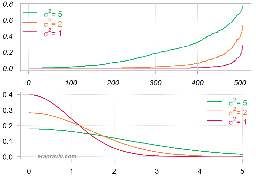
At the bottom I plot the (right) tail of the normal distribution with the corresponding $\sigma$ values. A high $\sigma$ value means that we are lenient in what we consider far. Put differently, there is a slower decay of the proximity score with respect to the distance. While a low $\sigma$ value means faster decay, so observations are quickly being considered different with every small drift away.

Everything written here is optional. There are many options you must consider. Distance metrics sure, but then also how to reverse them to similarities, and what is the chosen profile for the decay. You can tailor your own based on your application at hand. You don’t have to restrict yourself to what is baked into textbooks. You may want a different profile. For example a slow decay when observations are fairly close, faster decay thereafter, and again a slow decay for far away groups. Any profile that makes sense and obey the math is legitimate. I decided to invest time writing this post because downstream ML tasks (such as clustering for example) are quite sensitive to these underlying choices. Since many people, for whatever reason, gloss over those choices, this topic does not get enough attention. I think.