Are returns this year actually different than what can be expected from a typical year? Is the variance actually different than what can be expected from a typical year? Those are fairly light, easy to answer questions. We can use tests for equality of means or equality of variances.
But how about the following question:
is the profile\behavior of returns this year different than what can be expected in a typical year?
This is a more general and important question, since it encompasses all moments and tail behavior. And it is not as trivial to answer.
In this post I am scratching an itch I had since I wrote Understanding Kullback – Leibler Divergence. In the Kullback – Leibler Divergence post we saw how to quantify the difference between densities, exemplified using SPY return density per year. Once I was done with that post I was thinking there must be a way to test the difference formally, rather than just quantify, visualize and eyeball. And indeed there is. This post aim is to show to formally test for equality between densities.
There are in fact at least two ways in which you can test equality between two densities, or two distributions. The first is more classic. The test is called Kolmogorov–Smirnov test. The other is more modern, using permutation test (which requires simulation). We show both. Let’s first pull some price data:
|
1 2 3 4 5 6 7 8 9 10 11 12 13 14 15 16 17 18 19 20 21 22 23 24 25 26 |
library(quantmod) ; citation("quantmod") symetf = c('SPY') end<- format(Sys.Date(),"%Y-%m-%d") start<-"2006-01-01" l = length(symetf) dat0 <- lapply(symetf, getSymbols, src="yahoo", from=start, to=end, auto.assign = F,warnings = FALSE,symbol.lookup = F) xd <- dat0[[1]] timee <- index(xd) retd <- as.numeric(xd[2:NROW(xd),4])/as.numeric(xd[1:(NROW(xd)-1),4]) -1 tail(retd) # get the index up to 2018. # We later compare 2018 with the rest tmpind <- which(index(dat0[[1]])=="2017-12-29") # Mean and SD of daily returns (2018 excluded) > mean(100*retd[1:tmpind]) 0.0323 > sd(100*retd[1:tmpind]) 1.22 > # Mean and SD of daily returns in 2008 (so far) > mean(100*retd[-c(1:tmpind)]) 0.0459 > sd(100*retd[-c(1:tmpind)]) 0.888 |
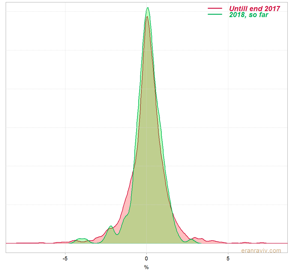
We can see that the mean and standard deviation of the daily returns for 2018 is a bit different than the mean and standard deviation of the rest. This is how the estimated densities look like:
Kolmogorov–Smirnov test
What we can do is compute the cumulative distribution function  for each of the densities. The one for 2018 and the one excluding 2018. Say distribution
  is for 2018 and distribution
  is for the rest. We compute the difference
  for each of the x’s. We know how the maximum of those (absolute) differences is distributed, so we can use that maximum as a test statistic, if it turns out too far out in the tails, we then decide the two distributions are different. Formally, but with a somewhat lax notation:
![\[\sqrt{n} \max_{x} \vert F_1(x)-F_2(x) \vert \xrightarrow {n\to \infty } \max _{t} \vert B(F(t))\vert\]](https://eranraviv.com/wp-content/ql-cache/quicklatex.com-6d535ae511b2c0265b844d2da9a7e74e_l3.svg "Rendered by QuickLaTeX.com")
where  is between 0 and 1 (by construction, since we subtract two probabilities and take the absolute value).
  is a Brownian bridge. It is not super interesting, all you should care about is that the (maximum of) the difference has a known distribution. This is a limit distribution, so we need a large number of observations, n, to have confidence in this test.
Kolmogorov-Smirnov test – R code
Let’s compare 2018 daily return with the rest of the returns to see if the distribution is the same based on the Kolmogorov-Smirnov test:
|
1 2 3 4 5 6 7 8 9 10 11 12 |
# Kolmogorov-Smirnov test #### ks.test(100*retd[1:tmpind], 100*retd[-c(1:tmpind)]) Two-sample Kolmogorov-Smirnov test data: 100 * retd[1:tmpind] and 100 * retd[-c(1:tmpind)] D = 0.067349, p-value = 0.3891 alternative hypothesis: two-sided Warning message: In ks.test(100 * retd[1:tmpind], 100 * retd[-c(1:tmpind)]) : p-value will be approximate in the presence of ties |
Fast and painless. We see that the maximum is 0.067 and that based on the limiting distribution the p-value is 0.3891. So no evidence that the distribution of 2018 is in any way different than the rest.
Let’s look at the permutation test. The main reason is that in order for the Kolmogorov-Smirnov test to be valid, given that it is based on a limiting distribution, we need a large number of observations. But nowadays we don’t have to rely on asymptotics as much as we had to in the past, because we can use computers.
Permutation test of equality between two densities
Intuitively, if the densities are exactly the same, we can bunch them together and sample from the “bunched data”. In our example, because we gathered the returns into one vector, permuting the vector implies that the daily returns from 2018 are now scattered across the vector, so taking a difference as in the equation above is like simulating from a null hypothesis: the distribution of 2018 daily returns is exactly the same as the rest. Now for each x we would have a difference under the null. We also have the actual difference for each x, from our observed data. We can now square (or take absolute values of) the actual difference between densities (per x), and compare it to our simulation results which were generated from the “bunched data”. The p-value can be estimated by looking at which quantile the actual difference falls within the simulated differences. If the actual data falls way outside the range of the distribution (of aggregated squared differences) under the null then we would reject the hypothesis that the distributions are the same.
Density comparison permutation test – R code
There is a fantastic package called sm (“sm” smoothing methods). There is also an accompanied book (see reference below).
We use the function sm.density.compare from that package to do what just described. The two argument nboot and ngrid are the number of simulation you would like to have and the number of grid points across the x you would like to use when you compute the . So ngrid=100 would “chop” the support into 100 points.
|
1 2 3 4 5 6 7 8 9 10 11 12 |
library("sm") citation("sm") # get help on the permutation test ?sm.density.compare # We need the index of the two groups, 2018 and the rest: ind1 <- substr(timee[-1], 1, 4) tmp_ind <- ind1 == 2018 sm.density.compare(100*retd, tmp_ind, model="equal", nboot= 500, ngrid= 100) Test of equal densities: p-value = 0.326 |
We can see that p-value is not very different than what we got using Kolmogorov-Smirnov test. This is how it looks like:
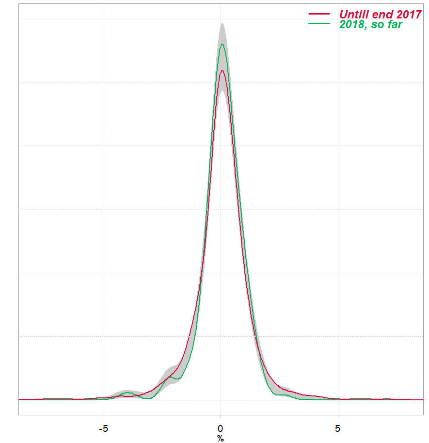
Of course, there is more nitty gritty to discuss, but the itch is gone.
Help me help you
References
Applied Smoothing Techniques for Data Analysis.


This is a very interesting package. In the plot resulting from sm.density.compare, how can you tell which line represents which group? How did you add the embelishments to the graph displayed here, like the key/legend? Thanks