Curse of dimensionality part 1: Value at Risk

The term ‘curse of dimensionality’ is now standard in advanced statistical courses, and refers to the disproportional increase in data which is needed to allow only slightly more complex models. This is true in high-dimensional settings. Here is an illustration of the ‘Curse of dimensionality’ in action.

‘Curse of dimensionality’ illustration; Value at risk estimation

There has been a tremendous and gratifying advances in the estimation of Value-at-Risk (VaR). Loosely speaking, this value is a lower-bound. With some probability, say 10%, and helped by some assumptions, you will lose no more than that particular value. For a single name in the portfolio, estimating a 10% VaR is fairly easy to do. What is important is that you have enough data for your estimate to be accurate. Specifically, it is crucial to have enough data points in that region- the 10% tail. The following figure shows the daily return distribution of US stocks (ticker SPY) and US bonds (ticker TLT). The blue bars represent points which lay in the 10% tail. Your VaR estimate relies heavily on those data points.

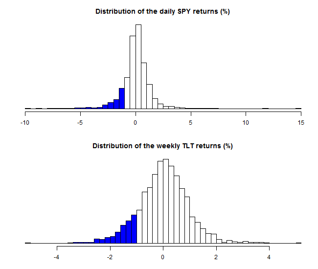
For 10 years of daily data we have 290 data points for SPY and 252 data points for TLT. A fair number, sure. Enough so that we can trust our VaR estimate (whichever you wish to estimate it).

Now, a lot of effort is flowing into the estimation of dependence in general, and specifically tail-dependence. You absolutely do not want your your bonds to fail you exactly when you rely the most on their protection\diversification. If there IS a strong tail dependence between stocks and bonds you need to find other instruments to defend your portfolio from tail event in stocks. But if tail-dependence is weak, really weak, not estimated to be weak, then you are good.

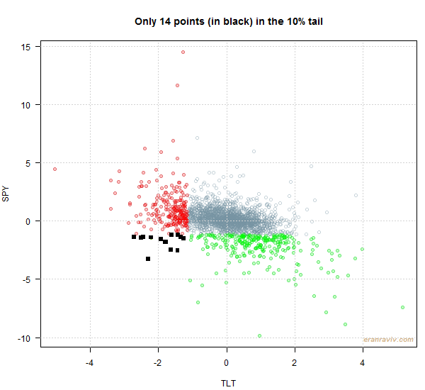
In the same spirit as for the (univariate) VaR estimation, for tail-dependence estimation you need enough data points so that you can estimate it reliably. Unlike the univariate case (VaR), now in the multivariate case, you need to have enough data points sitting elegantly in the 10% tail, but in the two dimensional space.

In the multivariate case much less of those around. See for yourself:

Only 14.

Quick calculation: if you would like to have roughly the same amount of data points comparable to what you had in the univariate case you need not 10 years of data, but ~180 years (250/14).

So estimating tail-dependence between say 4 variables, defining the tail as 5%… you need A LOT of data, otherwise ‘good luck to you sir’, estimation is just too fragile.

A classic text-book ‘curse of dimensionality’ figure and app

This practical example hints to a common picture typically shown whenever ‘curse of dimensionality’ is discussed (taken from newsnshit):

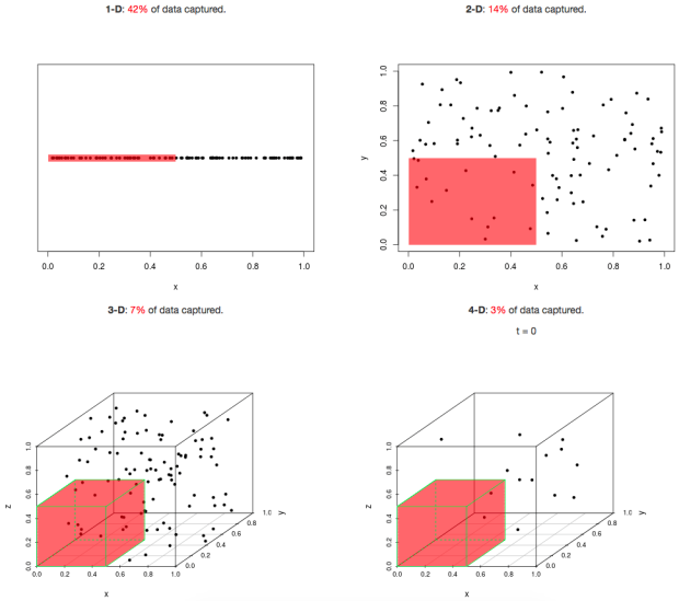
You can see that the number of data points that are captured by some fixed ‘length’ (in our previous example this is equivalent to the 10%) is rapidly diminishing as the dimension increases.

For a more interactive feel, where you can set your own ‘length’, check an shiny-app created by the guys from simplystatistics.

Code for (own) figures