Kullback - Leibler Divergence

It is easy to measure distance between two points. But what about measuring distance between two distributions? Good question. Long answer. Welcome the Kullback – Leibler Divergence measure.

The motivation for thinking about the Kullback – Leibler Divergence measure is that you can pick up questions such as: “how different was the behavior of the stock market this year compared with the average behavior?”. This is a rather different question than the trivial “how was the return this year compared to the average return?”.

It is very easy to measure distance between two points. But now we deal with whole distributions which somewhat complicates matters.

To discuss an explicit example, let’s start by plotting the distribution of daily returns on the S&P per year.

The code downloads data on the SPY ETF, calculates daily returns per year and estimates the densities. For the figure I use a [-5%, 5%] range for readability:


library(quantmod) ; citation("quantmod")
symetf = c('SPY')
end<- format(Sys.Date(),"%Y-%m-%d") 
start<-"2006-01-01"
l = length(symetf)
dat0 <- lapply(symetf, getSymbols,src="yahoo", from=start, to=end, auto.assign = F,warnings = FALSE,symbol.lookup = F)
names(dat0[[1]])
class((dat0[[1]]))
xd <- dat0[[1]]
head(xd)
timee <- index(xd)
retd <- as.numeric(xd[2:NROW(xd),4])/as.numeric(xd[1:(NROW(xd)-1),4]) -1
tail(retd)
# Compute the density per year:
dens <- density(retd)
ind1 <- substr(timee[-1], 1, 4) 
dens <- ind2 <- list()
for(i in 2006:2017){
ind2[[i]] <- i == ind1
dens[[i]] <- density(100*retd[ind2[[i]]])
}

library(quantmod) ; citation("quantmod")

symetf = c('SPY')

end<- format(Sys.Date(),"%Y-%m-%d")

start<-"2006-01-01"

l = length(symetf)

dat0 <- lapply(symetf, getSymbols,src="yahoo", from=start, to=end, auto.assign = F,warnings = FALSE,symbol.lookup = F)

names(dat0[[1]])

class((dat0[[1]]))

xd <- dat0[[1]]

head(xd)

timee <- index(xd)

retd <- as.numeric(xd[2:NROW(xd),4])/as.numeric(xd[1:(NROW(xd)-1),4]) -1

tail(retd)

# Compute the density per year:

dens <- density(retd)

ind1 <- substr(timee[-1], 1, 4)

dens <- ind2 <- list()

for(i in 2006:2017){

ind2[[i]] <- i == ind1

dens[[i]] <- density(100*retd[ind2[[i]]])

}

Distribution of daily returns per year

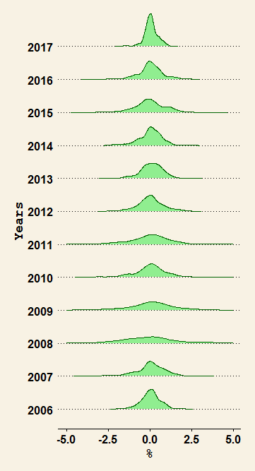
Those are the distributions of daily returns per year. What you can see is maybe something you know already, they are very different. We are on the way to quantify how different, to put a number of it.

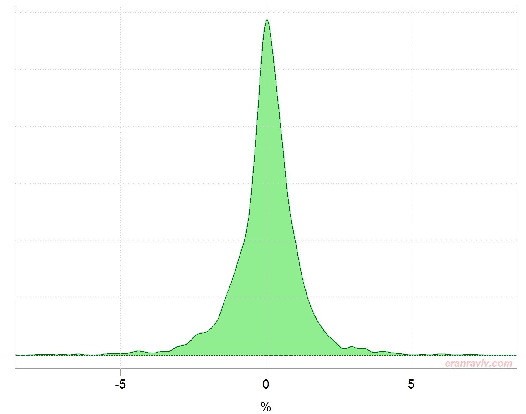
We can also plot the (estimate of the) density of the overall return distribution, up to 2017.

Distribution of daily returns excluding the year 2017

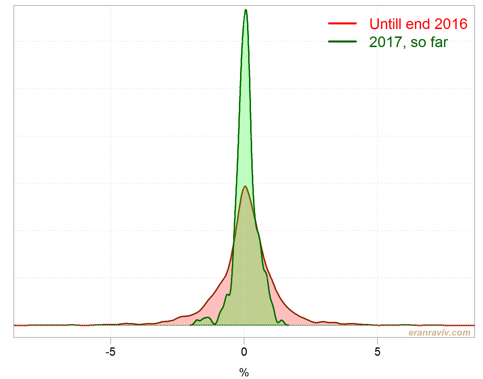
We can see the daily return distribution is different from one year to the next. Note the extreme heavy tails for some years. Simply eyeballing the figure above, the distribution for 2017 so far looks benevolent (tfo tfo) in comparison with the rest of the years. But we want to do better than eyeballing.

The Kullback – Leibler Divergence measure (KL from here onwards)

I too move uncomfortably in my chair pasting the next few formalities. Worry not, it will become clear in a sec.

For discrete probability distributions P and Q, the Kullback–Leibler divergence from Q to P is defined as:

${\displaystyle D_{\mathrm {KL} }(P\|Q)=-\sum _{i}P(i)\,\log {\frac {Q(i)}{P(i)}}}.$

which is equivalent to

${\displaystyle D_{\mathrm {KL} }(P\|Q)=\sum _{i}P(i)\,\log {\frac {P(i)}{Q(i)}}}.$

In words:

We have two distributions, Q and P. The distribution of say the daily returns during 2017, call it Q, and the overall distribution of daily return up until (excluding) 2017, call it P.

The measure is a sum.

We sum over i, which you can think about as the x-axis in the figures above.

The Q(i) is the density (an estimate of the density in practice) of the 2017 distribution at point i. The P(i) is the density (an estimate of the density in practice) of the overall distribution at point i. Note to self: at the same point i.

The log operator is standard in information theory, which is the origin of the KL Divergence measure.

The P(i) is key to understand this measure. Think about it as a weighting scheme. When i= roughly zero, the P(0) (estimate of the) density is quite high, so if there is a big difference around that point between the two distributions we give it a high weight in the overall measure. However, if we look at i= roughly 5, then the (estimate of the) P(5) density is quite low, so there can be a large difference between those distributions there without a large impact on the Kullback – Leibler measure. Only if you insist (as you do undoubtedly), another way to think about it is as an expectation of that ratio according to the P distribution.

From that last point we understand there must be a base-distribution call it. There is no analogy with scalars, there is no base-point from which you measure the distance between the two points. Stated clearly: the Kullback – Leibler measure is actually not a distance. Distance has few formal conditions. Symmetry is an important condition, and it does not hold here. If we interchange Q and P, such that Q is the overall distribution instead of the 2017 distribution, we would get a different number. This explains the use of the word divergence, rather than simply calling it distance. More in this promptly.

Let’s look at the two distributions jointly, the distribution of daily returns up to 2017, and the distribution of daily return during 2017 (up to now). I care about the shape, so I don’t mind what is on the y-axis.
Now lets compute the divergence between those two. We can use the LaplacesDemon package in R.


library("LaplacesDemon") # Install if not already
citation("LaplacesDemon")
tmpind <- which(index(dat0[[1]])=="2016-12-30")
density_tot <- density(100*retd[1:tmpind])
KL <- KLD(density_tot$y, dens[[2017]]$y)
plot(KL$KLD.py.px)

library("LaplacesDemon") # Install if not already

citation("LaplacesDemon")

tmpind <- which(index(dat0[[1]])=="2016-12-30")

density_tot <- density(100*retd[1:tmpind])

KL <- KLD(density_tot$y, dens[[2017]]$y)

plot(KL$KLD.py.px)

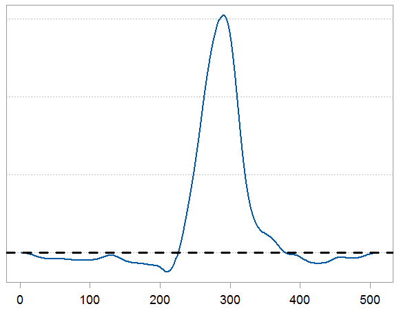
We have 500 points roughly. We can sum up those 500 points to get a KL summary measure for the divergence between those two distributions. This measure can be used as a quantification, but the chart is also useful when you want to know what and where exactly is the origin of the divergence. Also, we have some negative values which is fine. Think about the squared error metric, when you square an error smaller than 1 you actually make it smaller. Here when the ratio is below 1 it contribute negatively to the overall divergence. The sum however would never be negative. If the two distributions are the same then the sum should be zero. Although in practice it would not be because of estimation noise.

Next time you hear people say “those are special times” you now have a tool to quantify and check it.

Appendix

If Kullback – Leibler measure is not a distance, how should we think about it then?
One of my favorite bloggers lists possible interpretations for the Kullback – Leibler divergence measure:
The divergence from Y to X
The relative entropy of X with respect to Y
How well Y approximates X
The information gain going from the prior Y to the posterior X
The average surprise in seeing Y when you expected X